070: CFB Model

Data

table_games <- readRDS("2023_cfb_games.rds")

model_minutes <- readRDS("2023_cfb_model.rds")

Tufte Box Plot for Duration

table_games |> 
  ggplot2::ggplot(ggplot2::aes(x = week, y = minutes, group = week)) + 
  ggthemes::geom_tufteboxplot(stat = "boxplot", color = "floralwhite",
                              outlier.colour = "floralwhite",
                              outlier.shape = 21,
                              outlier.size = 0.5) + 
  hrbrthemes::theme_modern_rc() + 
  ggplot2::scale_x_continuous(breaks = seq(0, 15, 1)) + 
  ggplot2::scale_y_continuous(limits = c(0, 450), breaks = seq(0, 450, 50)) + 
  ggplot2::labs(x = "Week", y = "Minutes", 
                title = "2023 College Football Game Duration by Week", 
                subtitle = "The median game duration is about 200 minutes or 3 hours and 20 minutes",
                caption = "Bless your chart | data via sportsourceanalytics.com | January 17, 2024") + 
  ggplot2::annotate(
    "label",
    x = 5.3,
    y = 400,
    label = "More weather delays in early weeks!",
    size = 3.5,
    color = "#333333",
    family = "Roboto Condensed",
    fill = "floral white"
  ) +
  ggplot2::annotate(
    geom = "curve",
    color = "floralwhite",
    x = 2,
    y = 300,
    xend = 5.3,
    yend = 380,
    curvature = .3,
    arrow = ggplot2::arrow(length = grid::unit(2, "mm"))
  ) +
  ggplot2::annotate(
    geom = "curve",
    color = "floralwhite",
    x = 7,
    y = 200,
    xend = 10,
    yend = 100,
    curvature = -.3,
    arrow = ggplot2::arrow(length = grid::unit(2, "mm"))
    ) +
      ggplot2::annotate(
        "label",
        x = 10.5,
        y = 80,
        label = "Median game length ~200 minutes",
        size = 3.5,
        color = "#333333",
        family = "Roboto Condensed",
        fill = "floral white"
      ) -> min_plot 


ggplot2::ggsave(
  "min_plot.png",
  min_plot,
  w = 8,
  h = 6,
  dpi = 600,
  type = 'cairo'
) 

min_plot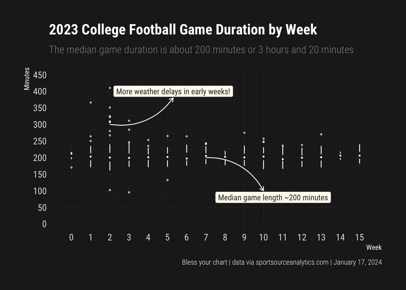

Model plot

# model <- parsnip::linear_reg() |>  
#  parsnip::set_engine("lm") |> 
#  generics::fit(minutes ~ total_drives + total_points 
#                + point_diff + total_plays + total_turnovers + 
#                  total_punts + total_rush_plays + total_incom + total_sp_td
#                + total_pens, data = kore_games)


# print(summary(model$fit))

# kore_games$est_minutes <- stats::predict(model, kore_games)


# model_minutes <- kore_games |> 
#  dplyr::mutate(est_duration = est_minutes[[".pred"]])

model_minutes |> 
  dplyr::filter(minutes < 300 & minutes > 150) |> 
  ggplot2::ggplot(ggplot2::aes(x = minutes, y = est_duration)) +
  ggplot2::geom_point(alpha = 0.5) +
  ggplot2::geom_abline(intercept = 0, slope = 1, color = "lightpink") +
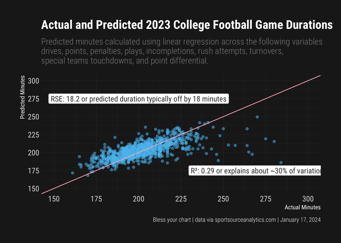
  ggplot2::labs(title = "Actual and Predicted 2023 College Football Game Durations",
                subtitle = "Predicted minutes calculated using linear regression across the following variables  \ndrives, points, penalties, plays, incompletions, rush attempts, turnovers,  \nspecial teams touchdowns, and point differential.",
                caption = "Bless your chart | data via sportsourceanalytics.com | January 17, 2024", 
                x = "Actual Minutes",
                y = "Predicted Minutes") + 
  ggplot2::scale_x_continuous(limits = c(150, 300), breaks = seq(150, 300, 25)) +
  ggplot2::scale_y_continuous(limits = c(150, 300), breaks = seq(150, 300, 25)) +
  hrbrthemes::theme_modern_rc() +
  ggplot2::annotate(
    geom = "label",
    x = 200,
    y = 275,
    family = "Roboto Condensed",
    label = "RSE: 18.2 or predicted duration typically off by 18 minutes",
    color = "#333333",
    size = 4,
  ) +
  ggplot2::annotate(
    geom = "label",
    x = 270,
    y = 175,
    family = "Roboto Condensed",
    label = "R²: 0.29 or explains about ~30% of variation",
    color = "#333333",
    size = 4,
  ) -> reg_plot 


ggplot2::ggsave(
  "reg_plot.png",
  reg_plot,
  w = 8,
  h = 8,
  dpi = 600,
  type = 'cairo'
) 
  
reg_plot