047: Drive chart

Load data

unc_drives <- readr::read_csv("unc_drives.csv") |> 
              dplyr::mutate(start_yd = dplyr::if_else(
                team_name == "North Carolina", 100-start_yd,
                start_yd
              ),
              end_yd = dplyr::if_else(
                team_name == "North Carolina", 100-end_yd,
                end_yd
              ),
              start_yd = dplyr::if_else(
                team_name == "Appalachian State", 100-start_yd,
                start_yd
              ),
              end_yd = dplyr::if_else(
                team_name == "Appalachian State", 100-end_yd,
                end_yd
              ))

app_color <- "#222222"
unc_color <- "#56a0d3"

unc_drive_colors <- c("Appalachian State" = app_color,
                  "North Carolina" = unc_color) 

unc_scoring_title <- "<span style='font-family: mono; fontface: bold'><span style='color:#56a0d3'>North Carolina 40</span><br>
<span style='color:#222222;'>Appalachian State 34</span><br>
Drive chart</span>" 

caption <- "<span style='font-family: mono; fontface: bold'> Excludes garbage time drives<br><br>
Bless your chart | data via SportSource Analytics</span>" 

only_unc <- unc_drives |> 
  dplyr::filter(team_name == "North Carolina") 

only_app <- unc_drives |> 
  dplyr::filter(team_name == "Appalachian State") 

## state drives
state_drives <- readr::read_csv("state_drives.csv") |> 
              dplyr::mutate(start_yd = dplyr::if_else(
                team_name == "Notre Dame", 100-start_yd,
                start_yd
              ),
              end_yd = dplyr::if_else(
                team_name == "Notre Dame", 100-end_yd,
                end_yd
              ),
              start_yd = dplyr::if_else(
                team_name == "North Carolina State", 100-start_yd,
                start_yd
              ),
              end_yd = dplyr::if_else(
                team_name == "North Carolina State", 100-end_yd,
                end_yd
              ))

nd_color <- "#C99700"
st_color <- "#CC0000"

state_drive_colors <- c("North Carolina State" = st_color,
                  "Notre Dame" = nd_color) 

state_scoring_title <- "<span style='font-family: mono; fontface: bold'><span style='color:#C99700'>Notre Dame 45</span><br>
<span style='color:#CC0000;'>NC State 24</span><br>
Drive chart</span>" 

only_state <- state_drives |> 
  dplyr::filter(team_name == "North Carolina State") 

only_nd <- state_drives |> 
  dplyr::filter(team_name == "Notre Dame") 

Set the theme

theme_me <- function() {
  # Create a base theme with minimal style
  base_theme <- ggplot2::theme_minimal(base_size = 10, base_family = "RobotoCondensed-Regular")
  
  # Customize the base theme with additional modifications
  custom_theme <- base_theme +
    ggplot2::theme(
      plot.title = ggplot2::element_text(
        hjust = 0.5,
        size = 24,
        face = "bold"
      ),
      plot.subtitle = ggplot2::element_text(
        hjust = 0.5,
        size = 10,
        lineheight = 0.25,
        vjust = -0.5
      ),
      plot.caption = ggplot2::element_text(
        hjust = 1,
        size = 6,
        lineheight = 0.35,
        margin = ggplot2::margin(t = 20)
      ),
      panel.grid.minor = ggplot2::element_line(color = "gray", linetype = "dotted"),  # Customize minor grid lines
      plot.background = ggplot2::element_rect(fill = "floralwhite", color = "floralwhite")
    )
  
  return(custom_theme)
} 

UNC drive plot

ggplot2::ggplot(unc_drives) +
  ggplot2::geom_segment(ggplot2::aes(x = drive_num, xend = drive_num, y = start_yd,
                        yend = end_yd, color = team_name), size = 1.5,
                        arrow = ggplot2::arrow(type = "closed", 
                                     length = ggplot2::unit(0.07, "inches"))) +
  ggplot2::scale_y_reverse(limits = c(120, -20), breaks = seq(-20, 120, 10),
                           labels = rev(c("", "", "0", "10", "20", "30", "40", "50",
                                      "40", "30", "20", "10", "0", "", ""))) +
  ggplot2::scale_x_reverse(limits = c(28, -4), breaks = seq(28, -4, -1), 
                              expand = c(0, -0.5)) +
  ggplot2::coord_flip() +
  ggplot2::scale_color_manual(values = unc_drive_colors) +
  theme_me() +
  ggplot2::theme(legend.position = "none", 
                 plot.title = ggtext::element_markdown(),
                 plot.caption = ggtext::element_markdown(),
                 panel.grid.major.x = ggplot2::element_line(color = "#E6E6E6", size = 0.5), 
                 panel.grid.minor.x = ggplot2::element_blank(),
                 panel.grid.major.y = ggplot2::element_blank(), 
                 panel.grid.minor.y = ggplot2::element_blank(),
                 axis.text.y = ggplot2::element_blank(),
                 axis.text.x = ggplot2::element_blank(),
                 axis.title.x = ggplot2::element_text(size = 14, face = "bold")) +
  ggplot2::geom_hline(yintercept = c(-10, -20, 110, 120), 
                      color = "floral white") +
  ggplot2::geom_vline(xintercept = 20.5, 
                      color = "#333333", linetype = "dashed") +
  ggplot2::labs(x = "",
                y = "Yard line",
                title = "",
                caption = caption) +
  ggplot2::annotate(
    geom = "label",
      x = only_unc$drive_num,
      y = -14,
    label =  paste(only_unc$result, "\n",
                   only_unc$plays, "plays", 
                   only_unc$yards, "yards"),
    color = "#333333",
    fill = "#56a0d3",
    size = 2.3,
    fontface = 'bold',
    family = 'mono',
    alpha = .3,
    hjust = 0.5
  ) +
    ggplot2::annotate(
      geom = "label",
      x = only_app$drive_num,
      y = 114,
      label =  paste(only_app$result, "\n",
                     only_app$plays, "plays", 
                     only_app$yards, "yards"),
      color = "#333333",
      fill = "#ffcc00",
      size = 2.3,
      fontface = 'bold',
      family = 'mono',
      alpha = .3,
      hjust = 0.5
    ) +
  ggplot2::annotate(
    cfbplotR::GeomCFBlogo,
    x = -2.5,
    y = -14,
    team = "North Carolina",
    height = .075,
  ) +
    ggplot2::annotate(
      "text",
      x = -0.5,
      y = -14,
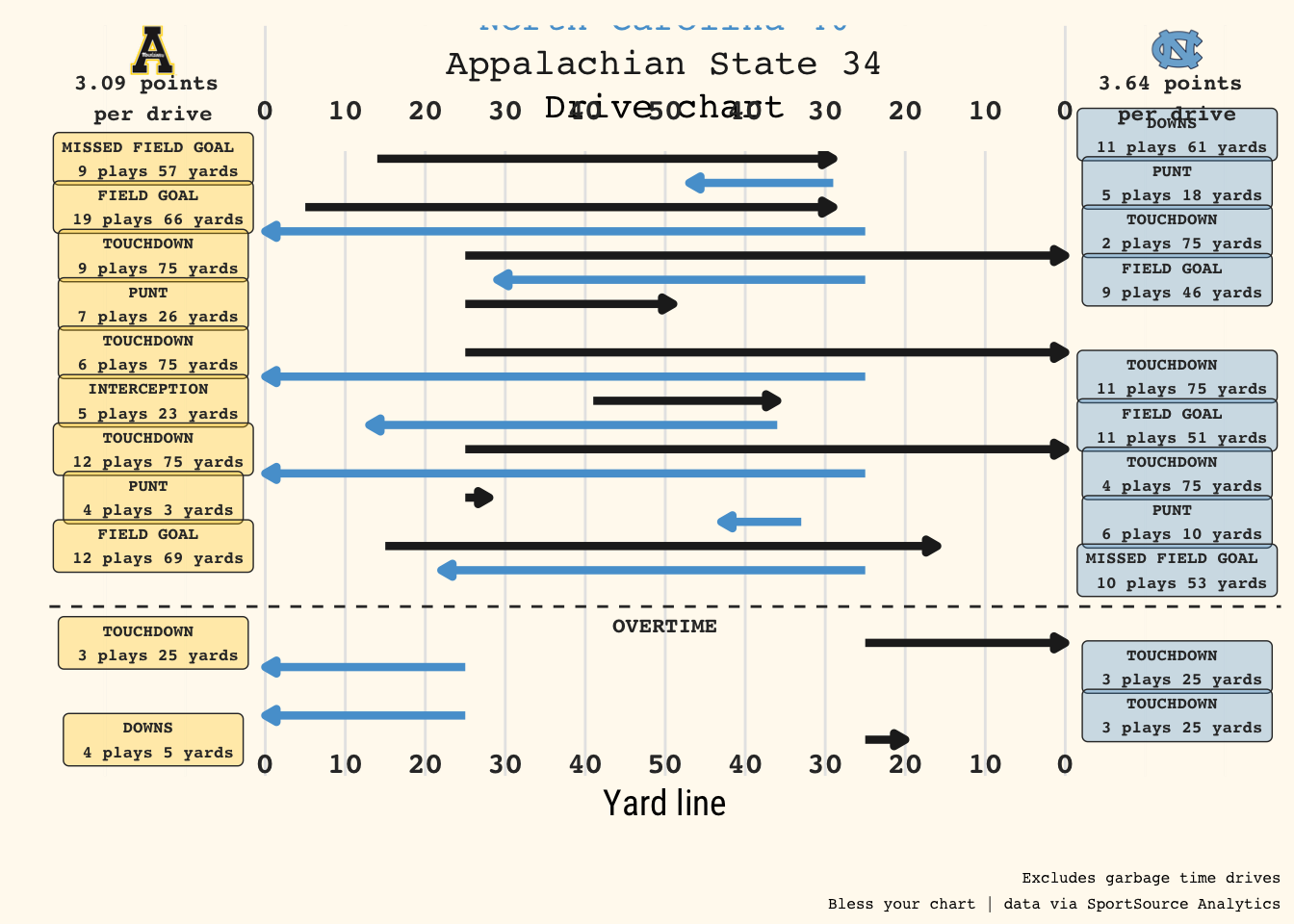
      label = " 3.64 points  \nper drive",
      fontface = 'bold',
      family = 'mono',
      size = 3,
      color = "#333333"
    ) +
    ggplot2::annotate(
      cfbplotR::GeomCFBlogo,
      x = -2.5,
      y = 114,
      team = "Appalachian State",
      height = .075,
    ) +
    ggplot2::annotate(
      "text",
      x = -0.5,
      y = 114,
      label = " 3.09 points  \nper drive",
      fontface = 'bold',
      family = 'mono',
      size = 3,
      color = "#333333",
    ) +
    ggplot2::annotate(
      "text",
      x = 21.3,
      y = 50,
      label = "OVERTIME",
      fontface = 'bold',
      family = 'mono',
      size = 3,
      color = "#333333",
    ) +
    ggtext::geom_richtext(
      x = 1.8,
      y = -50,
      label = unc_scoring_title,
      fill = "floral white", 
      label.color = NA,
      size = 5,
      label.padding = ggplot2::unit(c(0.7,4.5,0.7,4.5), "lines")
      ) + 
  ggplot2::annotate(
    geom = "text",
      x = 0,
      y = c(100, 90, 80, 70, 60, 50, 40, 30, 20, 10, 0),
    label =  c("0", "10", "20", "30", "40", "50",
               "40", "30", "20", "10", "0"),
    color = "#333333",
    size = 4,
    fontface = 'bold',
    family = 'mono',
    hjust = 0.5
  ) +
    ggplot2::annotate(
    geom = "text",
      x = 27.01,
      y = c(100, 90, 80, 70, 60, 50, 40, 30, 20, 10, 0),
    label =  c("0", "10", "20", "30", "40", "50",
               "40", "30", "20", "10", "0"),
    color = "#333333",
    size = 4,
    fontface = 'bold',
    family = 'mono',
    hjust = 0.5
  ) -> unc_drive_plot   

ggplot2::ggsave(
  "unc_drive_plot.png",
  unc_drive_plot,
  h = 8.65,
  w = 6.85,
  dpi = 600,
  type = 'cairo'
) 

unc_drive_plot

NC State drive plot

 state_drives |> 
 dplyr::filter(yards > -1) |>    
ggplot2::ggplot() +
  ggplot2::geom_segment(ggplot2::aes(x = drive_num, xend = drive_num, y = start_yd,
                        yend = end_yd, color = team_name), size = 1.5,
                        arrow = ggplot2::arrow(type = "closed", 
                                     length = ggplot2::unit(0.07, "inches"))) +
   ggplot2::geom_segment(data = state_drives |> 
                  dplyr::filter(yards < 0),
                ggplot2::aes(x = drive_num, xend = drive_num, y = end_yd,
                        yend = start_yd, color = team_name),
     size = 1.5, alpha = 0.3) +
  ggplot2::scale_y_reverse(limits = c(120, -20), breaks = seq(-20, 120, 10),
                           labels = rev(c("", "", "0", "10", "20", "30", "40", "50",
                                      "40", "30", "20", "10", "0", "", ""))) +
  ggplot2::scale_x_reverse(limits = c(34, -6), breaks = seq(34, -6, -1), 
                              expand = c(0, -1)) +
  ggplot2::coord_flip() +
  ggplot2::scale_color_manual(values = state_drive_colors) +
  theme_me() +
  ggplot2::theme(legend.position = "none", 
                 plot.title = ggtext::element_markdown(),
                 plot.caption = ggtext::element_markdown(),
                 panel.grid.major.x = ggplot2::element_line(color = "#E6E6E6", size = 0.5), 
                 panel.grid.minor.x = ggplot2::element_blank(),
                 panel.grid.major.y = ggplot2::element_blank(), 
                 panel.grid.minor.y = ggplot2::element_blank(),
                 axis.text.y = ggplot2::element_blank(),
                 axis.text.x = ggplot2::element_text(size = 12, 
                                                     face = "bold"),
                 axis.title.x = ggplot2::element_text(size = 14, face = "bold")
  ) +
  ggplot2::geom_hline(yintercept = c(-10, -20, 110, 120), 
                      color = "floral white") +
  ggplot2::labs(x = "",
                y = "Yard line",
                title = "",
                caption = caption) +
  ggplot2::annotate(
    geom = "label",
      x = only_state$drive_num,
      y = -14,
    label =  paste(only_state$result, "\n",
                   only_state$plays, "plays", 
                   only_state$yards, "yards"),
    color = "#333333",
    fill = st_color,
    size = 2.3,
    fontface = 'bold',
    family = 'mono',
    alpha = .3,
    hjust = 0.5
  ) +
    ggplot2::annotate(
      geom = "label",
      x = only_nd$drive_num,
      y = 114,
      label =  paste(only_nd$result, "\n",
                     only_nd$plays, "plays", 
                     only_nd$yards, "yards"),
      color = "#333333",
      fill = nd_color,
      size = 2.3,
      fontface = 'bold',
      family = 'mono',
      alpha = .3,
      hjust = 0.5
    ) +
  ggplot2::annotate(
    cfbplotR::GeomCFBlogo,
    x = -3.5,
    y = -14,
    team = "NC State",
    height = .075,
  ) +
    ggplot2::annotate(
      "text",
      x = -1.3,
      y = -14,
      label = " 1.6 points  \nper drive",
      fontface = 'bold',
      family = 'mono',
      size = 3,
      color = "#333333"
    ) +
    ggplot2::annotate(
      cfbplotR::GeomCFBlogo,
      x = -3.5,
      y = 114,
      team = "Notre Dame",
      height = .075,
    ) +
    ggplot2::annotate(
      "text",
      x = -1.3,
      y = 114,
      label = " 3.0 points  \nper drive",
      fontface = 'bold',
      family = 'mono',
      size = 3,
      color = "#333333",
    ) +
    ggtext::geom_richtext(
      x = 3,
      y = -50,
      label = state_scoring_title,
      fill = "floral white", 
      label.color = NA,
      size = 5,
      label.padding = ggplot2::unit(c(2,6,2,6), "lines")
      ) -> state_drive_plot   

ggplot2::ggsave(
  "state_drive_plot.png",
  state_drive_plot,
  h = 9.65,
  w = 6.85,
  dpi = 600,
  type = 'cairo'
) 

state_drive_plot