labels <- tejas |>
dplyr::group_by(rtg) |>
dplyr::filter(date == min(date) | date == max(date)) |>
dplyr::ungroup()
facet_labels <- c("kenpom" = "kenpom", "torvik" = "Torvik", "NET" = "NET")
date_breaks <- as.Date(c("2025-11-30", "2025-12-30", "2026-01-30"))
tejas_plot <- ggplot2::ggplot(tejas, ggplot2::aes(x = date, y = rank)) +
ggplot2::geom_line(linewidth = 0.8, color = "#bf5700") +
ggplot2::geom_point(data = labels,
size = 2.5,
color = "#bf5700") +
ggplot2::geom_text(
data = labels,
ggplot2::aes(label = rank),
vjust = -0.65,
hjust = -0.15,
size = 3.5,
fontface = "bold",
color = "#56a0d3"
) +
ggplot2::facet_wrap( ~ rtg, labeller = ggplot2::as_labeller(facet_labels)) +
ggplot2::scale_y_reverse(
limits = c(100, 1),
breaks = c(1, 25, 50, 75, 100),
expand = ggplot2::expansion(mult = c(0.05, 0.02))
) +
ggplot2::scale_x_date(
breaks = date_breaks,
labels = c("Nov 30", "Dec 30", "Jan 30"),
expand = ggplot2::expansion(mult = c(0.02, 0.08))
) +
hrbrthemes::theme_ipsum() +
ggplot2::labs(
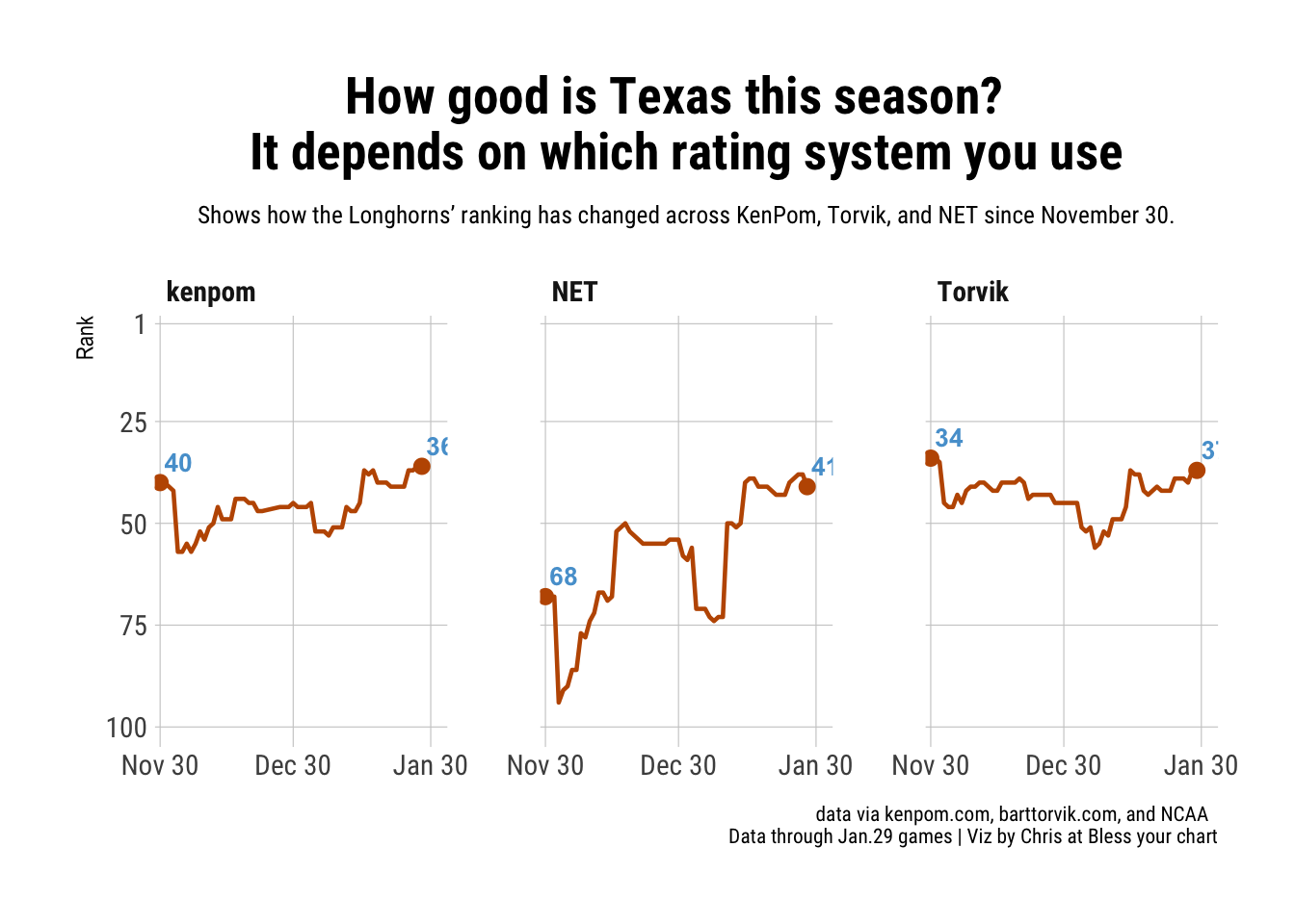
title = "How good is Texas this season? \nIt depends on which rating system you use",
subtitle = "Shows how the Longhorns' ranking has changed across KenPom, Torvik, and NET since November 30.",
x = NULL,
y = "Rank",
caption = "data via kenpom.com, barttorvik.com, and NCAA \nData through Jan.29 games | Viz by Chris at Bless your chart"
) +
ggplot2::theme(
plot.title = ggplot2::element_text(
hjust = 0.5,
size = 20,
family = "Roboto Condensed"
),
plot.subtitle = ggtext::element_markdown(
hjust = 0.5,
size = 9.5,
lineheight = 1.5,
family = "Roboto Condensed"
),
strip.text = ggplot2::element_text(
face = "bold",
size = 11,
family = "Roboto Condensed"
),
panel.grid.minor = ggplot2::element_blank(),
panel.spacing = ggplot2::unit(2.5, "lines"),
axis.text.x = ggplot2::element_text(size = 11, family = "Roboto Condensed"),
axis.text.y = ggplot2::element_text(size = 11, family = "Roboto Condensed"),
plot.caption = ggplot2::element_text(
face = "plain",
size = 8,
family = "Roboto Condensed"
)
)
ggplot2::ggsave("tejas_plot.png",
tejas_plot,
w = 10.5,
h = 7,
dpi = 600,
bg = "white",
type = "cairo")
tejas_plot