opponent_lists <- list(
"Penn State" = psu_opp[[2]],
"Ohio State" = osu_opp[[2]]
)
venn_plot <- ggvenn::ggvenn(
opponent_lists,
fill_color = c("#041E42", "#BB0000"), # Penn State navy and Ohio State scarlet
fill_alpha = 0.3,
stroke_size = 1.5,
set_name_size = 0,
show_elements = FALSE,
text_color = "#333333",
text_size = 4
) +
hrbrthemes::theme_ipsum_rc(base_family = "Roboto Condensed") +
ggplot2::labs(
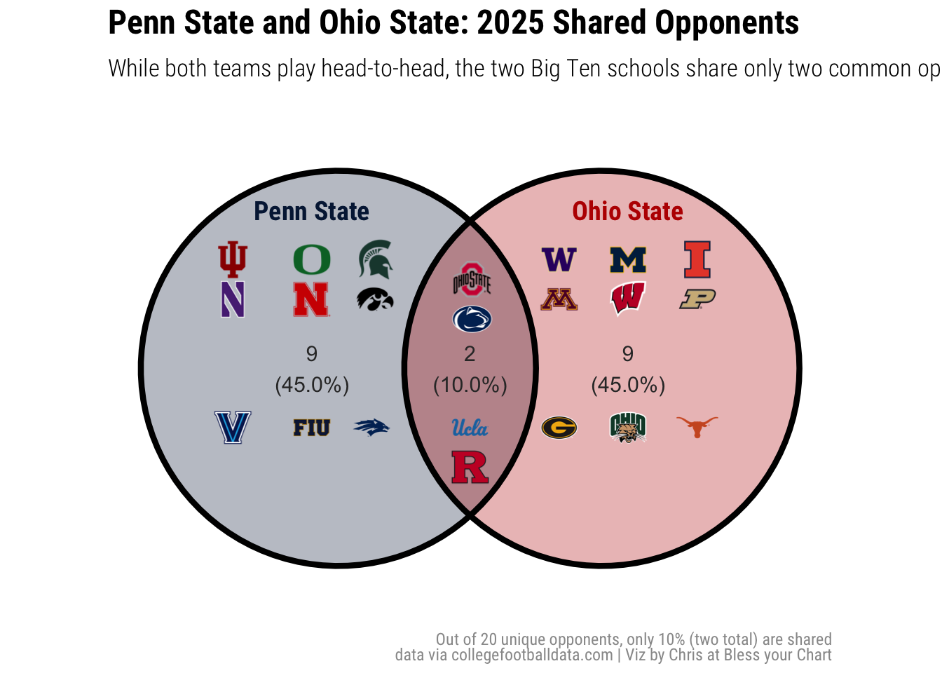
title = "Penn State and Ohio State: 2025 Shared Opponents",
subtitle = "While both teams play head-to-head, the two Big Ten schools share only two common opponents.",
x = "",
y = "",
caption = "Out of 20 unique opponents, only 10% (two total) are shared \ndata via collegefootballdata.com | Viz by Chris at Bless your Chart"
) +
ggplot2::theme(
text = ggplot2::element_text(family = "Roboto Condensed"),
plot.subtitle = ggtext::element_markdown(),
plot.caption = ggtext::element_markdown(color = "gray60",
family = "Roboto Condensed",
hjust = 1),
plot.margin = ggplot2::margin(t = 5, r = 20, b = 5, l = 5, unit = "pt"),
# Remove ALL axis elements including numbers
axis.title = ggplot2::element_blank(),
axis.text = ggplot2::element_blank(),
axis.text.x = ggplot2::element_blank(),
axis.text.y = ggplot2::element_blank(),
axis.ticks = ggplot2::element_blank(),
axis.line = ggplot2::element_blank(),
# Remove panel elements
panel.grid.major = ggplot2::element_blank(),
panel.grid.minor = ggplot2::element_blank(),
panel.border = ggplot2::element_blank(),
panel.background = ggplot2::element_blank(),
# Remove plot background
plot.background = ggplot2::element_blank(),
# Remove legend elements (if you want)
legend.background = ggplot2::element_blank(),
legend.key = ggplot2::element_blank(),
# Remove strip elements (for facets)
strip.background = ggplot2::element_blank(),
strip.text = ggplot2::element_blank()
) +
ggplot2::annotate(
cfbplotR::GeomCFBlogo,
x = 0,
y =-0.30,
team = "UCLA",
height = .085,
) +
ggplot2::annotate(
cfbplotR::GeomCFBlogo,
x = 0,
y =-0.50,
team = "Rutgers",
height = .085,
) +
ggplot2::annotate(
cfbplotR::GeomCFBlogo,
x = .01,
y = 0.25,
team = "Penn State",
height = .085,
) +
ggplot2::annotate(
cfbplotR::GeomCFBlogo,
x = 0.01,
y = 0.45,
team = "Ohio State",
height = .085,
) + # show penn st opponents
ggplot2::annotate(
cfbplotR::GeomCFBlogo,
x = -0.80,
y = 0.55,
team = "Oregon",
height = .085,
) +
ggplot2::annotate(
cfbplotR::GeomCFBlogo,
x = -1.2,
y = 0.55,
team = "Indiana",
height = .085,
) +
ggplot2::annotate(
cfbplotR::GeomCFBlogo,
x = -0.48,
y = 0.55,
team = "Michigan State",
height = .085,
) +
ggplot2::annotate(
cfbplotR::GeomCFBlogo,
x = -0.80,
y = 0.35,
team = "Nebraska",
height = .085,
) +
ggplot2::annotate(
cfbplotR::GeomCFBlogo,
x = -1.2,
y = 0.35,
team = "Northwestern",
height = .085,
) +
ggplot2::annotate(
cfbplotR::GeomCFBlogo,
x = -0.48,
y = 0.35,
team = "Iowa",
height = .085,
) +
ggplot2::annotate(
cfbplotR::GeomCFBlogo,
x = -0.8,
y = -0.30,
team = "Florida International",
height = .085,
) +
ggplot2::annotate(
cfbplotR::GeomCFBlogo,
x = -0.5,
y = -0.30,
team = "Nevada",
height = .085,
) +
ggplot2::annotate(
cfbplotR::GeomCFBlogo,
x = -1.2,
y = -0.30,
team = "Villanova",
height = .085,
) + # ohio state opponents
ggplot2::annotate(
cfbplotR::GeomCFBlogo,
x = 1.15,
y = -0.30,
team = "Texas",
height = .090,
) +
ggplot2::annotate(
cfbplotR::GeomCFBlogo,
x = 0.80,
y = -0.30,
team = "Ohio",
height = .085,
) +
ggplot2::annotate(
cfbplotR::GeomCFBlogo,
x = 0.45,
y = -0.30,
team = "Grambling",
height = .085,
) +
ggplot2::annotate(
cfbplotR::GeomCFBlogo,
x = 0.45,
y = 0.55,
team = "Washington",
height = .085,
) +
ggplot2::annotate(
cfbplotR::GeomCFBlogo,
x = 0.80,
y = 0.55,
team = "Michigan",
height = .085,
) +
ggplot2::annotate(
cfbplotR::GeomCFBlogo,
x = 1.15,
y = 0.55,
team = "Illinois",
height = .085,
) +
ggplot2::annotate(
cfbplotR::GeomCFBlogo,
x = 0.45,
y = 0.35,
team = "Minnesota",
height = .085,
) +
ggplot2::annotate(
cfbplotR::GeomCFBlogo,
x = 0.80,
y = 0.35,
team = "Wisconsin",
height = .085,
) +
ggplot2::annotate(
cfbplotR::GeomCFBlogo,
x = 1.15,
y = 0.35,
team = "Purdue",
height = .085,
) +
# Add team name annotations with Roboto Condensed font
ggplot2::annotate(
"text",
x = -0.8,
y = 0.8,
label = "Penn State",
family = "Roboto Condensed",
size = 5,
fontface = "bold",
color = "#041E42"
) +
ggplot2::annotate(
"text",
x = 0.8,
y = 0.8,
label = "Ohio State",
family = "Roboto Condensed",
size = 5,
fontface = "bold",
color = "#BB0000"
)
ggplot2::ggsave(
"vd_plot.png",
venn_plot,
w =10,
h = 8,
dpi = 600,
type = 'cairo',
bg = "white"
)
venn_plot