# sort out how to convert yards
convert_to_yards <- function(spot) {
team <- stringr::str_sub(spot, 1, 1)
yard <- as.numeric(stringr::str_sub(spot, 2, -1))
if (team == "B") {
return(yard)
} else {
return(100 - yard)
}
}
# figure out how ball moves
ball_movement <- drives_raw |>
dplyr::mutate(
drive_num = dplyr::row_number(),
start_yd = purrr::map_dbl(Drive_Started_Spot, convert_to_yards),
end_yd = purrr::map_dbl(Drive_Ended_Spot, convert_to_yards),
team_name = Team,
quarter = Qtr
)
bmadj <- ball_movement |>
dplyr::mutate(
is_touchdown = stringr::str_detect(How_Lost, "TOUCHDOWN") |
(team_name == "BC" & end_yd >= 100) |
(team_name == "ND" & end_yd <= 0),
is_points = is_touchdown | stringr::str_detect(How_Lost, "Field Goal"),
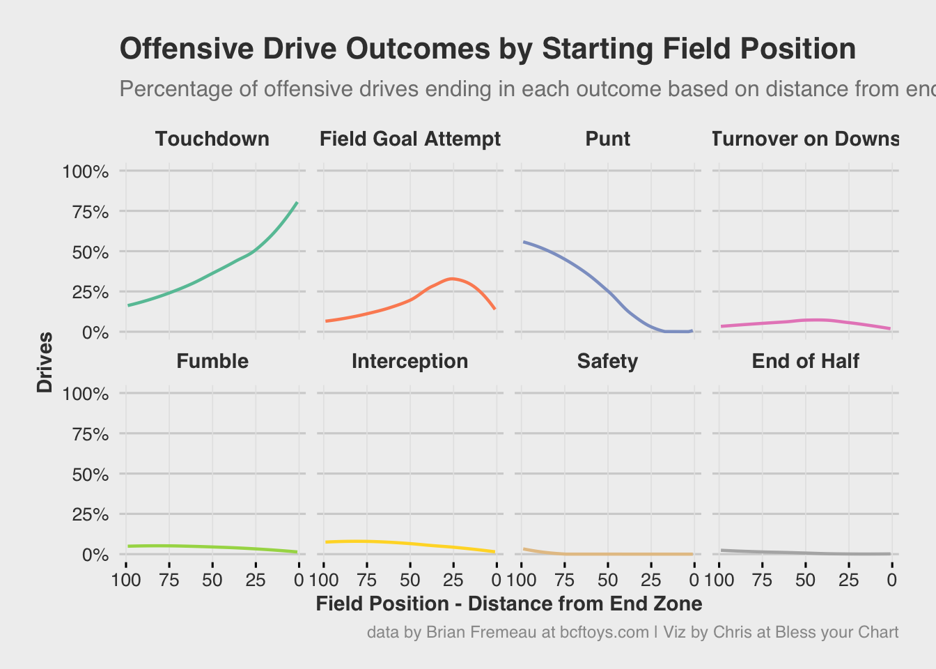
drive_outcome = dplyr::case_when(
is_touchdown ~ "Touchdown",
stringr::str_detect(How_Lost, "Field Goal") ~ "Field Goal",
stringr::str_detect(How_Lost, "Punt") ~ "Punt",
stringr::str_detect(How_Lost, "Fumble") ~ "Fumble",
stringr::str_detect(How_Lost, "Interception") ~ "Interception",
stringr::str_detect(How_Lost, "Downs") ~ "Turnover on Downs",
TRUE ~ "Other"
)
)
# Create start and end points with outcome info
start_points <- data.frame(
possession = 1:nrow(bmadj),
position = bmadj$start_yd,
point_type = "Drive Start",
team = bmadj$team_name,
outcome = "Start",
is_touchdown = FALSE,
is_points = FALSE
)
end_points <- data.frame(
possession = 1:nrow(bmadj),
position = bmadj$end_yd,
point_type = "Drive End",
team = bmadj$team_name,
outcome = bmadj$drive_outcome,
is_touchdown = bmadj$is_touchdown,
is_points = bmadj$is_points
)
all_points <- rbind(start_points, end_points)
# Create shape mapping with directional triangles
all_points <- all_points |>
dplyr::mutate(
shape_type = dplyr::case_when(
point_type == "Drive Start" & team == "BC" ~ "BC Start",
point_type == "Drive Start" & team == "ND" ~ "ND Start",
point_type == "Drive End" & is_touchdown ~ "Touchdown",
point_type == "Drive End" & is_points ~ "Points",
point_type == "Drive End" & !is_points ~ "No Points"
)
)
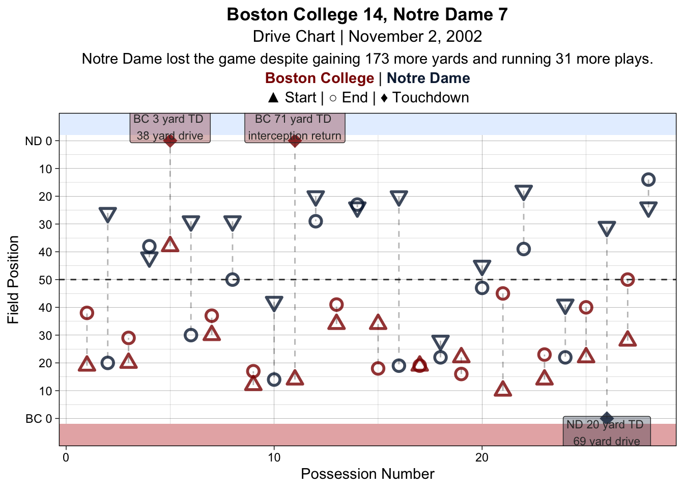
bc_nd_plot <- ggplot2::ggplot(
all_points,
ggplot2::aes(x = possession, y = position)
) +
ggplot2::geom_line(
ggplot2::aes(group = possession),
alpha = 0.3,
linetype = "dashed"
) +
ggplot2::geom_point(
ggplot2::aes(color = team, shape = shape_type, size = shape_type),
alpha = 0.8,
stroke = 1.5
) +
ggplot2::scale_color_manual(values = c("BC" = "#8B0000", "ND" = "#0C2340")) +
ggplot2::geom_rect(
ggplot2::aes(xmin = -Inf, xmax = Inf, ymin = 102, ymax = 110),
fill = "#E6F0FF",
) +
ggplot2::geom_rect(
ggplot2::aes(xmin = -Inf, xmax = Inf, ymin = -10, ymax = -2),
fill = "#E7B3B3"
) +
ggplot2::scale_shape_manual(
values = c(
"BC Start" = 24, # up triangle is BC
"ND Start" = 25, # down triangle is ND
"No Points" = 1, # open circle
"Points" = 16, # closed circle
"Touchdown" = 18 # diamond
),
name = ""
) +
ggplot2::scale_size_manual(
values = c(
"BC Start" = 3,
"ND Start" = 3,
"No Points" = 3,
"Points" = 3,
"Touchdown" = 4
),
guide = "none"
) +
ggplot2::scale_y_continuous(
limits = c(-10, 110),
expand = c(0, 0),
breaks = seq(0, 100, 10),
labels = c(
"BC 0",
"10",
"20",
"30",
"40",
"50",
"40",
"30",
"20",
"10",
"ND 0"
)
) +
ggplot2::labs(
title = "**Boston College 14, Notre Dame 7**<br><span style='font-size:12pt'>Drive Chart | November 2, 2002</span>",
subtitle = "Notre Dame lost the game despite gaining 173 more yards and running 31 more plays.<br><span style='color:#8B0000'>**Boston College**</span> | <span style='color:#0C2340'>**Notre Dame**</span><br>▲ Start | ○ End | ♦ Touchdown",
x = "Possession Number",
y = "Field Position",
color = ""
) +
ggplot2::theme_linedraw() +
ggplot2::theme(
plot.title = ggtext::element_markdown(hjust = 0.5, lineheight = 1.2),
plot.subtitle = ggtext::element_markdown(hjust = 0.5, lineheight = 1.3),
legend.position = "none"
) +
ggplot2::annotate(
geom = "label",
x = 11,
y = 105,
label = "BC 71 yard TD \ninterception return",
color = "#333333",
fill = "#8B0000",
size = 3,
alpha = .3,
hjust = 0.5
) +
ggplot2::annotate(
geom = "label",
x = 5,
y = 105,
label = "BC 3 yard TD \n38 yard drive",
color = "#333333",
fill = "#8B0000",
size = 3,
alpha = .3,
hjust = 0.5
) +
ggplot2::annotate(
geom = "label",
x = 26,
y = -5,
label = "ND 20 yard TD \n69 yard drive",
color = "#333333",
fill = "#0C2340",
size = 3,
alpha = .3,
hjust = 0.5
) +
ggplot2::geom_hline(yintercept = 50, linetype = "dashed",
color = "#333333")
bc_nd_plot