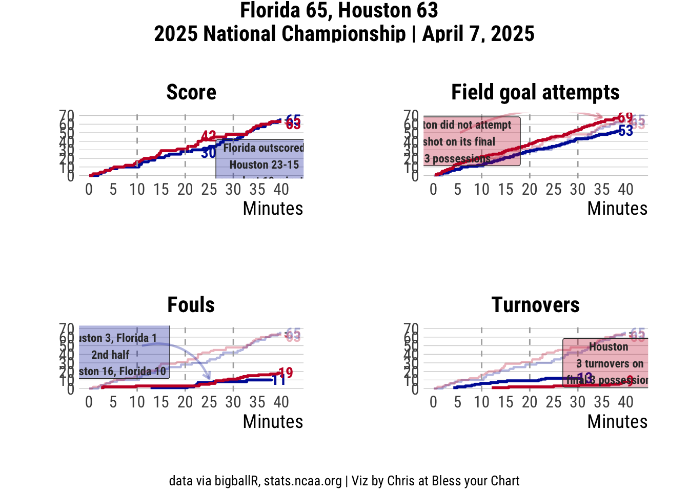
# schedule <- bigballR::get_team_schedule(team.name="Houston",season="2024-25") # pbp_hou <- bigballR::get_play_by_play(schedule$Game_ID[40]) <- readr:: read_csv ("pbp_houston.csv" )# set teams <- "Houston" <- "Florida" <- "#C8102E" <- "#0021A5" <- pbp_hou |> :: select (Game_Seconds, Home_Score, Away_Score) |> :: distinct () |> :: rename (secs_elapsed = Game_Seconds) |> :: pivot_longer (cols = c (Home_Score, Away_Score),names_to = "team" ,values_to = "score" |> :: mutate (team = dplyr:: case_when (== "Home_Score" ~ "Houston" ,== "Away_Score" ~ "Florida" # Field Goal Attempt data <- pbp_hou |> :: filter (Event_Type %in% c ("Three Point Jumper" , "Two Point Jumper" , "Layup" , "Hook" , "Dunk" )) |> :: mutate (team = dplyr:: case_when (== home_team ~ home_team,== away_team ~ away_team|> :: group_by (team) |> :: arrange (Game_Seconds, .by_group = TRUE ) |> :: mutate (fga_count = dplyr:: row_number ()) |> :: ungroup () |> :: rename (secs_elapsed = Game_Seconds)# Foul data <- pbp_hou |> :: filter (Event_Type == "Commits Foul" ) |> :: mutate (team = dplyr:: case_when (== home_team ~ home_team,== away_team ~ away_team|> :: group_by (team) |> :: arrange (Game_Seconds, .by_group = TRUE ) |> :: mutate (foul_count = dplyr:: row_number ()) |> :: ungroup () |> :: rename (secs_elapsed = Game_Seconds)# Turnovers <- pbp_hou |> :: filter (Event_Type == "Turnover" ) |> :: mutate (team = dplyr:: case_when (== home_team ~ home_team,== away_team ~ away_team|> :: group_by (team) |> :: arrange (Game_Seconds, .by_group = TRUE ) |> :: mutate (foul_count = dplyr:: row_number ()) |> :: ungroup () |> :: rename (secs_elapsed = Game_Seconds)# theme <- function () {:: theme_ipsum (base_family = "Roboto Condensed" ,grid = "Y" ,plot_title_size = 16 ,subtitle_size = 12 ,axis_title_size = 14 ,base_size = 12 + :: theme (plot.title = ggplot2:: element_text (hjust = 0.5 , face = "bold" ),plot.subtitle = ggplot2:: element_text (hjust = 0.5 ),axis.title = ggplot2:: element_text (),plot.caption = ggplot2:: element_text (size = 8 ),legend.position = "none" ,panel.grid.major.x = ggplot2:: element_blank (),panel.grid.minor.x = ggplot2:: element_blank (),plot.background = ggplot2:: element_rect (fill = "white" , color = "white" )# Score Plot <- ggplot2:: ggplot (score_data, ggplot2:: aes (x = secs_elapsed / 60 , y = score, color = team)) + :: geom_line (size = 1 ) + :: labs (x = "Minutes" ,y = "" ,color = "" ,title = "Score" + my_theme () + :: scale_color_manual (values = c (Houston = home_col, Florida = away_col)+ :: scale_x_continuous (breaks = seq (0 , max (score_data$ secs_elapsed, na.rm = TRUE ) / 60 , 5 )+ :: scale_y_continuous (breaks = seq (0 , 70 , 10 ), limits = c (0 , 70 )+ :: geom_vline (xintercept = c (10 , 20 , 30 ),linetype = "dashed" ,color = "#acacac" ) + :: annotate (:: GeomCFBlogo,x = 40.9 ,y = 65 ,team = "Florida" ,height = .055 + :: annotate (:: GeomCFBlogo,x = 40.9 ,y = 61 ,team = "Houston" ,height = .055 + :: annotate (geom = "text" ,x = 42.5 ,y = 65 ,color = away_col,label = "65" ,size = 4 ,fontface = 'bold' ,family = 'Roboto Condensed' + :: annotate (geom = "text" ,x = 42.5 ,y = 61 ,color = home_col,label = "63" ,size = 4 ,fontface = 'bold' ,family = 'Roboto Condensed' + :: annotate (geom = "text" ,x = 24.9 ,y = 27.6 ,color = away_col,label = "30" ,size = 4 ,fontface = 'bold' ,family = 'Roboto Condensed' + :: annotate (geom = "text" ,x = 24.9 ,y = 46.5 ,color = home_col,label = "42" ,size = 4 ,fontface = 'bold' ,family = 'Roboto Condensed' + :: annotate (geom = "label" ,x = 37 ,y = 13.5 ,color = "#333333" ,fill = away_col,label = "Florida outscored \n Houston 23-15 \n over last 10 minutes" ,size = 3 ,fontface = 'bold' ,family = 'Roboto condensed' ,alpha = 0.3 # Field Goal Attempts Plot <- ggplot2:: ggplot (score_data, ggplot2:: aes (x = secs_elapsed / 60 , y = score, color = team)) + :: geom_line (size = .75 , alpha = 0.3 ) + :: labs (x = "Minutes" ,y = "" ,color = "" ,title = "Field goal attempts" + my_theme () + :: scale_color_manual (values = c (Houston = home_col, Florida = away_col)+ :: scale_x_continuous (breaks = seq (0 , max (score_data$ secs_elapsed, na.rm = TRUE ) / 60 , 5 )+ :: scale_y_continuous (breaks = seq (0 , 70 , 10 ), limits = c (0 , 70 )+ :: geom_vline (xintercept = c (10 , 20 , 30 ),linetype = "dashed" ,color = "#acacac" ) + :: annotate (:: GeomCFBlogo,x = 40.9 ,y = 65 ,team = "Florida" ,height = .055 + :: annotate (:: GeomCFBlogo,x = 40.9 ,y = 61 ,team = "Houston" ,height = .055 + :: annotate (geom = "text" ,x = 42.5 ,y = 65 ,color = away_col,label = "65" ,size = 4 ,fontface = 'bold' ,family = 'Roboto Condensed' ,alpha = 0.3 + :: annotate (geom = "text" ,x = 42.5 ,y = 61 ,color = home_col,label = "63" ,size = 4 ,fontface = 'bold' ,family = 'Roboto Condensed' ,alpha = 0.3 + :: annotate (geom = "text" ,x = 40 ,y = 53 ,color = away_col,label = "53" ,size = 4 ,fontface = 'bold' ,family = 'Roboto Condensed' + :: annotate (geom = "text" ,x = 39.9 ,y = 69 ,color = home_col,label = "69" ,size = 4 ,fontface = 'bold' ,family = 'Roboto Condensed' + :: geom_step (data = fga_data,:: aes (x = secs_elapsed / 60 , y = fga_count, color = team),size = 1 + :: annotate (geom = "label" ,x = 5 ,y = 40 ,color = "#333333" ,fill = home_col,label = "Houston did not attempt \n a shot on its final \n 3 possessions" ,size = 3 ,fontface = 'bold' ,family = 'Roboto condensed' ,alpha = 0.3 + :: annotate (geom = "curve" ,color = home_col,x = 5.5 ,y = 50 ,xend = 35 ,yend = 68 ,curvature = - .2 ,linewidth = 0.8 ,arrow = ggplot2:: arrow (length = ggplot2:: unit (2 , "mm" )),alpha = 0.3 # Fouls Plot <- ggplot2:: ggplot (score_data, ggplot2:: aes (x = secs_elapsed / 60 , y = score, color = team)) + :: geom_line (size = .75 , alpha = 0.3 ) + :: labs (x = "Minutes" ,y = "" ,color = "" ,title = "Fouls" + my_theme () + :: scale_color_manual (values = c (Houston = home_col, Florida = away_col)+ :: scale_x_continuous (breaks = seq (0 , max (score_data$ secs_elapsed, na.rm = TRUE ) / 60 , 5 )+ :: scale_y_continuous (breaks = seq (0 , 70 , 10 ), limits = c (0 , 70 )+ :: geom_vline (xintercept = c (10 , 20 , 30 ),linetype = "dashed" ,color = "#acacac" ) + :: annotate (:: GeomCFBlogo,x = 40.9 ,y = 65 ,team = "Florida" ,height = .055 + :: annotate (:: GeomCFBlogo,x = 40.9 ,y = 61 ,team = "Houston" ,height = .055 + :: annotate (geom = "text" ,x = 42.5 ,y = 65 ,color = away_col,label = "65" ,size = 4 ,fontface = 'bold' ,family = 'Roboto Condensed' ,alpha = 0.3 + :: annotate (geom = "text" ,x = 42.5 ,y = 61 ,color = home_col,label = "63" ,size = 4 ,fontface = 'bold' ,family = 'Roboto Condensed' ,alpha = 0.3 + :: annotate (geom = "text" ,x = 39.5 ,y = 11 ,color = away_col,label = "11" ,size = 4 ,fontface = 'bold' ,family = 'Roboto Condensed' + :: annotate (geom = "text" ,x = 40.9 ,y = 19 ,color = home_col,label = "19" ,size = 4 ,fontface = 'bold' ,family = 'Roboto Condensed' + :: geom_step (data = foul_data,:: aes (x = secs_elapsed / 60 , y = foul_count, color = team),size = 1 + :: annotate (geom = "label" ,x = 5 ,y = 50 ,color = "#333333" ,fill = away_col,label = "1st half \n Houston 3, Florida 1 \n 2nd half \n Houston 16, Florida 10" ,size = 3 ,fontface = 'bold' ,family = 'Roboto condensed' ,alpha = 0.3 + :: annotate (geom = "curve" ,color = away_col,x = 11 ,y = 50 ,xend = 25 ,yend = 11.5 ,curvature = - .4 ,linewidth = 0.8 ,arrow = ggplot2:: arrow (length = ggplot2:: unit (2 , "mm" )),alpha = 0.3 # Turnovers Plot <- ggplot2:: ggplot (score_data, ggplot2:: aes (x = secs_elapsed / 60 , y = score, color = team)) + :: geom_line (size = .75 , alpha = 0.3 ) + :: labs (x = "Minutes" ,y = "" ,color = "" ,title = "Turnovers" + my_theme () + :: scale_color_manual (values = c (Houston = home_col, Florida = away_col)+ :: scale_x_continuous (breaks = seq (0 , max (score_data$ secs_elapsed, na.rm = TRUE ) / 60 , 5 )+ :: scale_y_continuous (breaks = seq (0 , 70 , 10 ), limits = c (0 , 70 )+ :: geom_vline (xintercept = c (10 , 20 , 30 ),linetype = "dashed" ,color = "#acacac" ) + :: annotate (:: GeomCFBlogo,x = 40.9 ,y = 65 ,team = "Florida" ,height = .055 + :: annotate (:: GeomCFBlogo,x = 40.9 ,y = 61 ,team = "Houston" ,height = .055 + :: annotate (geom = "text" ,x = 42.5 ,y = 65 ,color = away_col,label = "65" ,size = 4 ,fontface = 'bold' ,family = 'Roboto Condensed' ,alpha = 0.3 + :: annotate (geom = "text" ,x = 42.5 ,y = 61 ,color = home_col,label = "63" ,size = 4 ,fontface = 'bold' ,family = 'Roboto Condensed' ,alpha = 0.3 + :: annotate (geom = "text" ,x = 31.5 ,y = 13 ,color = away_col,label = "13" ,size = 4 ,fontface = 'bold' ,family = 'Roboto Condensed' + :: annotate (geom = "text" ,x = 40.9 ,y = 9.5 ,color = home_col,label = "9" ,size = 4 ,fontface = 'bold' ,family = 'Roboto Condensed' + :: geom_step (data = to_data,:: aes (x = secs_elapsed / 60 , y = foul_count, color = team),size = 1 + :: annotate (geom = "label" ,x = 37 ,y = 30 ,color = "#333333" ,fill = home_col,label = "Houston \n 3 turnovers on \n final 3 possessions" ,size = 3 ,fontface = 'bold' ,family = 'Roboto condensed' ,alpha = 0.3 # grid <- cowplot:: plot_grid (ncol = 2 , align = "hv" # title <- cowplot:: ggdraw () + :: draw_label ("Florida 65, Houston 63 \n 2025 National Championship | April 7, 2025" , fontface = 'bold' , size = 16 , hjust = 0.5 ,fontfamily = "Roboto Condensed" # title to grid <- cowplot:: plot_grid (ncol = 1 ,rel_heights = c (0.1 , 1 )# footer <- cowplot:: ggdraw () + :: draw_label ("data via bigballR, stats.ncaa.org | Viz by Chris at Bless your Chart" , size = 10 , hjust = 0.5 , fontfamily = "Roboto Condensed" ,<- cowplot:: plot_grid (ncol = 1 ,rel_heights = c (1 , 0.05 ) # Footer is 5% height 


