138: Trends

Load data

library(rlang)
library(cbbplotR)
options(chromote.headless = "new")

# ------- Continuity data 
# yrs <- c(2010:2025)

# rm <- function(id) {
#  hoopR::kp_height(min_year = id, max_year = id) |>  
#    dplyr::mutate(season = id) |> 
#    dplyr::select(season, ncaa_seed, team, continuity, 
#                  continuity_rk, bench, bench_rk, experience, experience_rk) 
# }


# rm_data <- lapply(yrs, rm)

# rm_results <- as.data.frame(do.call(rbind, rm_data))


# transofrm data
# median_stats_long <- rm_results |>
#  dplyr::group_by(season) |>
#  dplyr::summarise(
#    `Experience (years)` = median(experience, na.rm = TRUE),
#    `Continuity (minutes)` = median(continuity, na.rm = TRUE)
#  ) |>
#  tidyr::pivot_longer(cols =
#                        c(`Experience (years)`, 
#                          `Continuity (minutes)`), 
#                      names_to = "Metric", 
#                      values_to = "Value")

cont_data <- readr::read_csv("cont_stats.csv")

# ---------- Shot profile data, big assist from cobrastats on player logs from Torvik 
shot_profile <- readr::read_csv("shot_profile.csv")

# ---------- UNC data 
unc <- readr::read_csv("unc_data.csv")

# manually add in other numbers from sports-refernece and wikipedia 

acct <- c(1981, 1982, 1989, 1991, 1994, 1997, 1998, 2007, 2008, 2016)

rs <- c(1982, 1983, 1984, 1985, 1987, 1988, 1993, 1995, 2001, 2005, 
        2007, 2008, 2009, 2011, 2012, 2016, 2017, 2019, 2024)

f4 <- c(1981, 1982, 1991, 1993, 1995, 1997, 1998, 2000, 2005, 2008, 2009, 2016, 2017, 2022)

titles <- c(1982, 1993, 2005, 2009, 2017)

nba <- c(1980, 1981, 1982, 1984, 1984, 1986, 1987, 1987, 1989, 1991, 1991,
         1992, 1993, 1994, 1995, 1995, 1998, 1998, 2001, 2001, 2005, 2005,
         2005, 2005, 2007, 2009, 2009, 2009, 2010, 2012, 2012, 2012, 2012, 
         2013, 2014, 2016, 2017, 2017, 2019, 2019, 2019, 2020, 2021)
         
# function to count by decade 
convert_to_decade <- function(years) {
  paste0(floor(years / 10) * 10, "s")
}

decade_counts <- data.frame(
  Decade = unique(c(convert_to_decade(acct), convert_to_decade(rs), convert_to_decade(f4), convert_to_decade(titles)))
) |>
  dplyr::mutate(
    ACCT = sapply(Decade, function(d) sum(convert_to_decade(acct) == d)),
    RS = sapply(Decade, function(d) sum(convert_to_decade(rs) == d)),
    F4 = sapply(Decade, function(d) sum(convert_to_decade(f4) == d)),
    Titles = sapply(Decade, function(d) sum(convert_to_decade(titles) == d)),
    NBA = sapply(Decade, function(d) sum(convert_to_decade(nba) == d)),
  ) |>
  dplyr::arrange(Decade)

# summarize the data
unc_summary <- unc |>
  dplyr::filter(Year > 1979) |> 
  dplyr::mutate(
    Decade = paste0(floor(Year / 10) * 10, "s")  # Convert Year to decade format
  ) |>
  dplyr::group_by(Decade) |>
  dplyr::summarize(
    Total_Wins = sum(W...6, na.rm = TRUE),
    Total_Losses = sum(L, na.rm = TRUE),
    Win_Percentage = Total_Wins / (Total_Wins + Total_Losses)
  ) |>
  dplyr::arrange(Decade)

# summarize the win percentages in a list 
unc_with_decade <- unc |>
  dplyr::filter(Year > 1979) |> 
  dplyr::mutate(
    Decade = paste0(floor(Year / 10) * 10, "s")  # Convert Year to decade format
  ) |>
  dplyr::group_by(Decade) |>
  dplyr::summarize(
    Yearly_Win_Pcts = list(rev(winpct))  # Store win percentages as a list per decade
  ) |>
  dplyr::arrange(Decade)

# all the tables 
unc_hist <- unc_summary |> 
  dplyr::left_join(decade_counts, by = "Decade") |> 
  dplyr::left_join(unc_with_decade, by = "Decade")

UNC decades table

heels_header <- glue::glue(
  "<div style='display: flex; justify-content: space-between; align-items: center;'>
      <div>
       <img src='https://a.espncdn.com/combiner/i?img=/i/teamlogos/ncaa/500/153.png'
       style='height: 55px; width: auto; vertical-align: middle;'>
     </div>
     <div style='flex-grow:1; margin-left: 30px; margin-right: 30px'>
       <span style='display: block; font-weight: bold; text-align: center; font-size: 24px;'>Carolina hoops over the past five decades</span>
       <span style='font-size: 12.5px; font-weight: normal; display: block; text-align: center;'>Performance across the ACC, NCAA Tournament, and overall win percentage.</span>
     </div>
     <div>
       <img src='https://a.espncdn.com/combiner/i?img=/redesign/assets/img/icons/ESPN-icon-basketball.png' 
       style='height: 45px; width: auto; vertical-align: middle;'>
     </div>
   </div>
  <br>"
)


unc_decade_tbl <- unc_hist |> 
  dplyr::mutate(record = paste0(Total_Wins, "-", Total_Losses)) |> 
  dplyr::relocate(Win_Percentage, .after = Titles) |>
  dplyr::relocate(NBA, .after = Decade) |>
  dplyr::mutate(
    Titles = dplyr::case_when(
    Titles %% 1 == 0 ~ strrep("trophy,", Titles),
    Titles %% 1 != 0 ~ paste0(strrep("trophy,", floor(Titles)), "trophy"))
  ) |> 
  gt::gt() |> 
  gtUtils::gt_theme_gtutils() |> 
  gt::fmt_icon(
    columns = c(Titles),
    rows = c(1, 2, 3, 4),
    fill_color = "orange"
  ) |> 
  gt::cols_hide(columns = c(Total_Wins, Total_Losses, NBA)) |> 
  gt::fmt_number(Win_Percentage, decimals = 3) |> 
  gtExtras::gt_merge_stack(
    col1 = Win_Percentage,
    col2 = record,
    palette = c("black", "#333333")
  ) |> 
  gtUtils::gt_column_subheaders(
    Win_Percentage = list(heading = "Win %", subtitle = "W-L"),
    #NBA = list(heading = "1st Round", subtitle = "# of Picks"),
    ACCT = list(heading = "Tournament", subtitle = "Titles"),
    RS = list(heading = "Regular", subtitle = "Season"),
    F4 = list(heading = "Final Fours", subtitle = "# of times"),
    Titles = list(heading = "Titles", subtitle = "# of titles"),
    heading_color = "black",
    subtitle_color = "gray"
  ) |> 
  gt::tab_spanner(
    columns = c(ACCT, RS),
    label = "ACC Championships"
  ) |> 
  gt::tab_spanner(
    columns = c(F4, Titles),
    label = "NCAA Tournament"
  ) |> 
  #gt::tab_spanner(
  #  columns = NBA,
  #  label = "NBA Draft"
  #) |> 
  gt::cols_label(
    Decade = ""
  ) |> 
  gt::cols_nanoplot(
    columns = Yearly_Win_Pcts,
    reference_line = .70,
    autohide = TRUE,
    plot_type = "line",
    new_col_label = "Over time",
    options = gt::nanoplot_options(
      data_area_fill_color = "#56a0d3",
      reference_line_color = "#333333",
      show_data_area = TRUE,
      show_data_points = FALSE
    )
  ) |> 
  gt::tab_header(title = gt::html(heels_header)) |>
  gt::tab_source_note(source_note = gt::html("<hr>Over time column shows win percentage by season throughout the decade (dashed line indicates a .700 win percentage).<br>Decades include the season's final year (i.e. 2019-20 is part of the 2020s)<hr><br><b>Table by Chris at Bless your Chart | data via sports-reference.com | April 4, 2025</b>")) |> 
  gt::data_color(
    columns = c(NBA, ACCT, RS, F4, Win_Percentage),
    direction = c("column"),
    method = c("numeric"),
    palette = c("#d7191c", "#fdae61", 
                "#ffffbf", "#a6d96a", 
                "#1a9641"),
    alpha = 0.6
  ) |>
  gt::tab_style(
    locations = gt::cells_column_labels(),
    style = gt::cell_text(
      font = gt::google_font("Signika Negative"),
      weight = "650",
      size = gt::px(14)
    )
  ) |> 
  gt::tab_style(
    locations = gt::cells_body(columns = Decade),
    style = gt::cell_text(
      font = gt::google_font("Signika Negative"),
      weight = "bold"
    )
  ) |> 
  gt::tab_style(
    locations = gt::cells_column_spanners(),
    style = gt::cell_text(
      font = gt::google_font("Signika Negative"),
      weight = 850,
      size = gt::px(14)
    )
  ) |>
  gt::tab_style(
    locations = gt::cells_source_notes(),
    style = gt::cell_text(
      font = gt::google_font("Signika Negative"),
      size = gt::px(11.5),
      weight = 250
    )
  ) |>
  gtUtils::gt_border_grid(color = "black",
                          weight = 2,
                          include_labels = FALSE) |> 
  gtUtils::gt_border_bars_bottom(c("#56a0d3", "#89BDE0", "#BBD9ED")) |> 
  gt::tab_options(table.width = gt::px(700))


gtUtils::gt_save_crop(
  unc_decade_tbl,
  file = "unc_decade_tbl.png",
  whitespace = 60,
  bg = "#FFFDF5"
)

unc_decade_tbl

Carolina hoops over the past five decades Performance across the ACC, NCAA Tournament, and overall win percentage.
	ACC Championships		NCAA Tournament		Win % W-L	Over time
	Tournament Titles	Regular Season	Final Fours # of times	Titles # of titles
1980s	3	6	2		0.817 281-63
1990s	4	2	5		0.776 270-78
2000s	2	5	4		0.728 251-94
2010s	1	5	2		0.743 277-96
2020s	0	1	1		0.639 133-75
Over time column shows win percentage by season throughout the decade (dashed line indicates a .700 win percentage). Decades include the season's final year (i.e. 2019-20 is part of the 2020s) Table by Chris at Bless your Chart | data via sports-reference.com | April 4, 2025

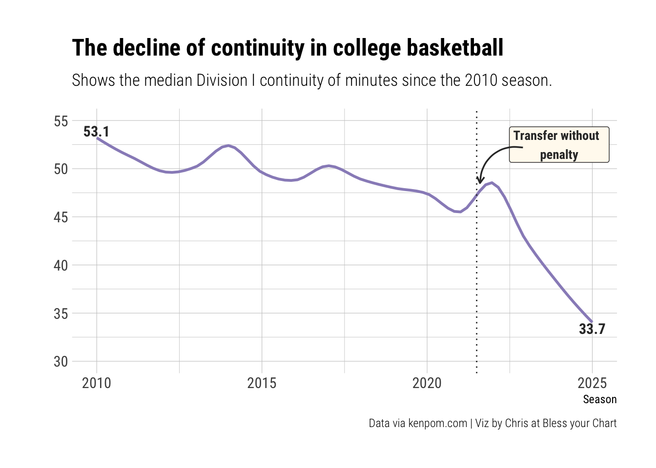
Continuity plot

cont_plot <- cont_data |> 
   dplyr::filter(Metric == "Continuity (minutes)") |> 
  ggplot2::ggplot(ggplot2::aes(x = season, y = Value, color = Metric)) +
  ggplot2::geom_smooth(method = "loess", se = FALSE, span = 0.35) +
  ggplot2::geom_vline(xintercept = 2021.5, linetype = "dotted", color = "#333333", linewidth = 0.5) +
  ggplot2::scale_color_manual(values = 
                                c("Continuity (minutes)" = "#998ec3")) +
  hrbrthemes::theme_ipsum_rc() +
  ggplot2::labs(
    title = "The decline of continuity in college basketball",
    subtitle = "Shows the median Division I continuity of minutes since the 2010 season.",
    x = "Season",
    y = "",
    caption ="Data via kenpom.com | Viz by Chris at Bless your Chart"
  ) +
  ggplot2::scale_y_continuous(limits = c(30, 55), 
                              breaks = seq(30, 55, 5)) +
  ggplot2::theme(legend.position = "none") +
  ggplot2::annotate(
    geom = "label",
    x = 2024,
    y = 52.5,
    color = "#333333",
    fill = "floralwhite",
    label = "Transfer without  \npenalty",
    size = 3.5,
    fontface = 'bold',
    family = 'Roboto condensed'
  ) +
  ggplot2::annotate(
    geom = "curve",
    color = "#333333",
    x = 2022.9,
    y = 52.2,
    xend = 2021.6,
    yend = 48.5,
    curvature = .5,
    linewidth = 0.6,
    arrow = ggplot2::arrow(length = ggplot2::unit(2, "mm"))
  ) +
  ggplot2::annotate(
    geom = "text",
    x = 2025,
    y = 33.4,
    color = "#333333",
    label = "33.7",
    size = 4,
    fontface = 'bold',
    family = 'Roboto condensed'
  ) +
  ggplot2::annotate(
    geom = "text",
    x = 2010,
    y = 53.9,
    color = "#333333",
    label = "53.1",
    size = 4,
    fontface = 'bold',
    family = 'Roboto condensed'
  )

ggplot2::ggsave(
  "cont_plot.png",
  cont_plot,
  w = 7.5,
  h = 6.5,
  dpi = 600,
  bg = "white",
  type = 'cairo'
)

cont_plot

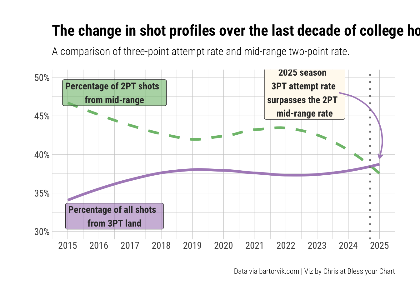
Mid-range plot

mr_plot <- shot_profile |> 
  dplyr::filter(season > 2014) |> 
  tidyr::pivot_longer(cols = c(mid_two_rate, three_rate), 
                      names_to = "shot_type", 
                      values_to = "rate") |> 
  ggplot2::ggplot(ggplot2::aes(x = season, y = rate, color = shot_type,
                               linetype = shot_type)) +
  ggplot2::geom_smooth(method = "loess", se = FALSE, linewidth = 1.5) +
  ggplot2::scale_color_manual(values = c("mid_two_rate" = "#7fbf7b", 
                                         "three_rate" = "#af8dc3")) +
  ggplot2::scale_linetype_manual(values = c("mid_two_rate" = "dashed", 
                                            "three_rate" = "solid")) +
  ggplot2::labs(title = "Shot Selection Trends Over Time",
                x = "",
                y = "",
                color = "Shot Type") +
  hrbrthemes::theme_ipsum_rc() +
  ggplot2::labs(
    title = "The change in shot profiles over the last decade of college hoops",
    subtitle = "A comparison of three-point attempt rate and mid-range two-point rate.",
    x = "",
    y = "",
    caption ="Data via bartorvik.com | Viz by Chris at Bless your Chart"
  ) +
  ggplot2::scale_x_continuous(limits = c(2015, 2025), 
                              breaks = seq(2015, 2025, 1)) +
  ggplot2::scale_y_continuous(
    limits = c(0.30, 0.50), 
    breaks = seq(0.30, 0.50, 0.05),
    labels = scales::percent_format(accuracy = 1)
  ) +
  ggplot2::theme(legend.position = "none") +
  ggplot2::annotate(
    geom = "label",
    x = 2016.5,
    y = .32,
    color = "#333333",
    fill = "#af8dc3",
    label = "Percentage of all shots  \nfrom 3PT land",
    size = 4,
    fontface = 'bold',
    family = 'Roboto condensed',
    alpha = 0.6
  ) +
  ggplot2::annotate(
    geom = "label",
    x = 2016.5,
    y = .48,
    color = "#333333",
    fill = "#7fbf7b",
    label = "Percentage of 2PT shots  \nfrom mid-range",
    size = 4,
    fontface = 'bold',
    family = 'Roboto condensed',
    alpha = 0.6
  ) +
  ggplot2::annotate(
    geom = "label",
    x = 2022.6,
    y = .48,
    color = "#333333",
    fill = "floralwhite",
    label = "2025 season  \n3PT attempt rate \nsurpasses the 2PT  \nmid-range rate",
    size = 4,
    fontface = 'bold',
    family = 'Roboto condensed'
  ) +
  ggplot2::annotate(
    geom = "curve",
    color = "#af8dc3",
    x = 2023.7,
    y = .48,
    xend = 2025,
    yend = .395,
    curvature = -.5,
    linewidth = 0.8,
    arrow = ggplot2::arrow(length = ggplot2::unit(2, "mm"))
  ) +
  ggplot2::geom_vline(xintercept = 2024.7, linetype = "dotted", color = "gray50", linewidth = 1)
  
ggplot2::ggsave(
  "mr_plot.png",
  mr_plot,
  w = 8.5,
  h = 7,
  dpi = 600,
  bg = "white",
  type = 'cairo'
)

mr_plot