library(rlang)library(cbbplotR)options(chromote.headless ="new")# this data is used in the evidence app, saving as a csv for static generation # https://github.com/gallochris/evdev-byc/blob/main/data/college-basketball/wab_logs.Rteam_sched_by_wab <- readr::read_csv("team_sched_by_wab.csv")quad_fun <- team_sched_by_wab |> dplyr::filter(quad =="Q1") |> dplyr::filter(team %in%c("North Carolina", "Indiana", "Gonzaga")) |> dplyr::mutate(location =factor(location, levels =c("H", "A", "N"))) |> dplyr::group_by(team) |> dplyr::mutate(wins =sum(result =="W"),games = dplyr::n(),win_pct = wins / games,total_wab =sum(wab_result),avg_bub_win_prob =mean(bub_win_prob),team_label =sprintf("%s\n(%d-%d)", team, wins, games - wins) ) |> dplyr::filter(games >1) |> dplyr::ungroup() |> dplyr::mutate(team_label = forcats::fct_reorder(team_label, win_pct))
Q1 Plot
Code
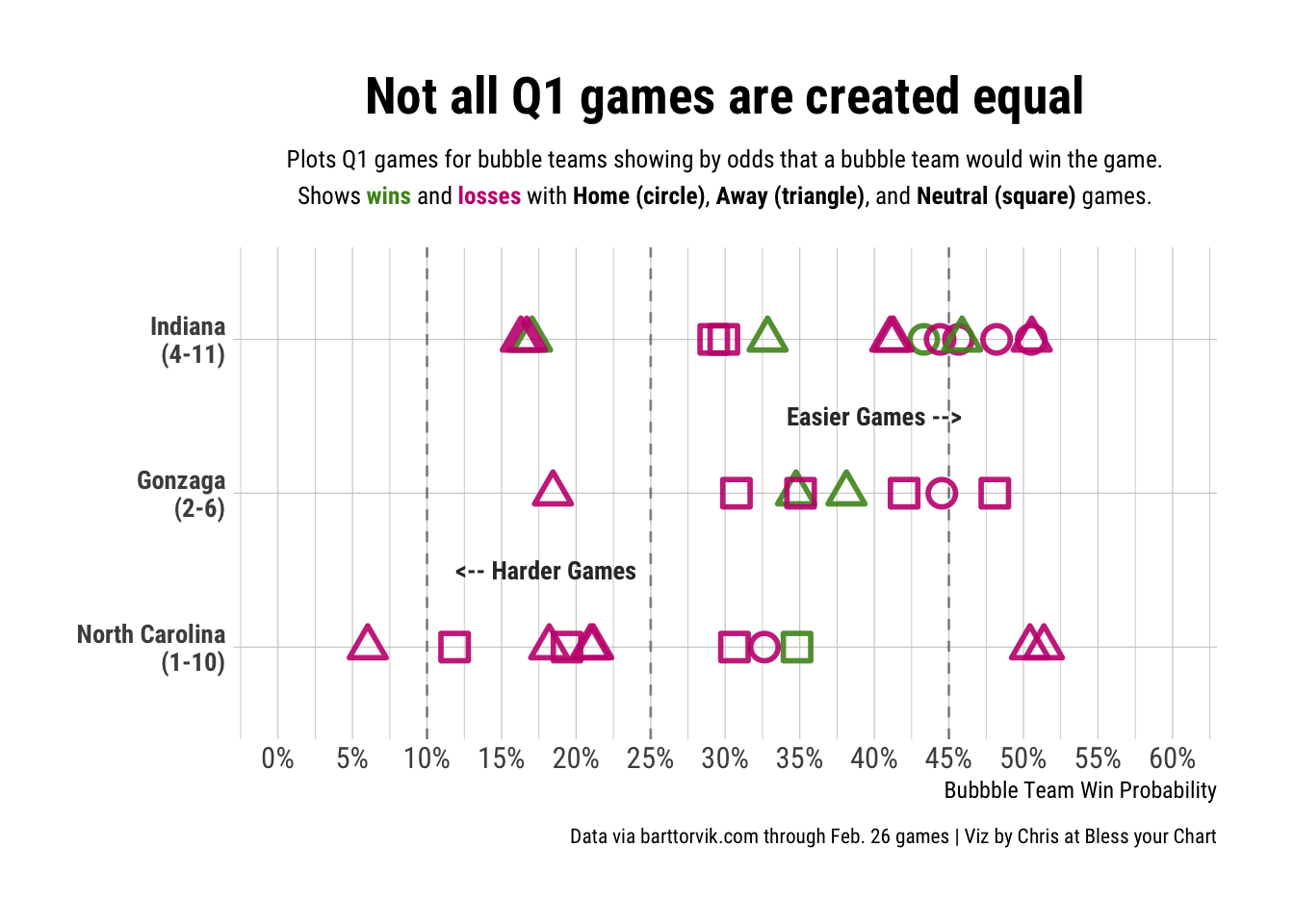
q1_plot <- quad_fun |> ggplot2::ggplot(ggplot2::aes(x = bub_win_prob, y = team_label, shape = location, color = result)) + ggplot2::geom_vline(xintercept =c(0.1, .25, .45), linetype ="dashed", color ="#333333", alpha =0.5) + ggplot2::geom_point(size =4, stroke =1.5, alpha =0.9, position = ggplot2::position_jitter(width =0.02, height =0) ) + ggplot2::scale_shape_manual(values =c("H"=1, "A"=2, "N"=0), name ="Location",labels =c("Home", "Away", "Neutral") ) + ggplot2::scale_color_manual(values =c("W"="#4d9221", "L"="#c51b7d"),name ="Result",labels =c("Win", "Loss") ) + ggplot2::labs(x ="Bubbble Team Win Probability", y =NULL, title ="Not all Q1 games are created equal",subtitle ="Plots Q1 games for bubble teams showing by odds that a bubble team would win the game.<br>Shows <span style='color: #4d9221;'><b>wins</span></b> and <span style='color: #c51b7d;'><b>losses</span></b> with <b>Home (circle)</b>, <b>Away (triangle)</b>, and <b>Neutral (square)</b> games.",caption ="Data via barttorvik.com through Feb. 26 games | Viz by Chris at Bless your Chart" ) + ggplot2::scale_x_continuous(limits =c(0, .60),breaks =seq(0, .60, .05),labels = scales::percent ) + ggplot2::annotate("text",x = .18,y =1.5,label ="<-- Harder Games",size =3.5,color ="#333333",family ="Roboto Condensed",fontface ="bold" ) + ggplot2::annotate("text",x = .40,y =2.5,label ="Easier Games -->",size =3.5,color ="#333333",family ="Roboto Condensed",fontface ="bold" ) + hrbrthemes::theme_ipsum_rc() + ggplot2::theme(plot.title = ggplot2::element_text(hjust =0.5,size =20,family ="Roboto Condensed" ),plot.subtitle = ggtext::element_markdown(hjust =0.5,size =9.5,lineheight =1.5,family ="Roboto Condensed" ),legend.position ="none",axis.text.y = ggplot2::element_text(size =10, family ="Roboto Condensed",face ="bold"),plot.caption = ggplot2::element_text(face ="plain", size =8, "Roboto Condensed") ) ggplot2::ggsave("q1_plot.png", q1_plot,w =8.5,h =6.5,dpi =600,bg ="white",type ='cairo')q1_plot
Play-by-play data
Code
# commenting out the functions here, so it easier to load the static data # game_set <- # bigballR::get_team_schedule(season = "2024-25", team.name = "North Carolina")# play_by_play <- bigballR::get_play_by_play(game_set$Game_ID)play_by_play <- readr::read_csv("play_by_play.csv")
New names:
Rows: 504 Columns: 36
── Column specification
──────────────────────────────────────────────────────── Delimiter: "," chr
(21): Date, Home, Away, Event_Team, Event_Description, Player_1, Player... dbl
(11): ...1, ID, Half_Status, Game_Seconds, Home_Score, Away_Score, Shot... lgl
(2): isTransition, isGarbageTime time (2): Time, Game_Time
ℹ Use `spec()` to retrieve the full column specification for this data. ℹ
Specify the column types or set `show_col_types = FALSE` to quiet this message.
• `` -> `...1`
New names:
Rows: 6 Columns: 8
── Column specification
──────────────────────────────────────────────────────── Delimiter: "," chr
(2): label_group, category dbl (6): ...1, PercentMins, NETRTG, ORTG, DRTG,
ORBper
ℹ Use `spec()` to retrieve the full column specification for this data. ℹ
Specify the column types or set `show_col_types = FALSE` to quiet this message.
• `` -> `...1`
New names:
Rows: 87 Columns: 5
── Column specification
──────────────────────────────────────────────────────── Delimiter: "," chr
(2): opp, category dbl (3): ...1, date, mins
ℹ Use `spec()` to retrieve the full column specification for this data. ℹ
Specify the column types or set `show_col_types = FALSE` to quiet this message.
• `` -> `...1`
Lineup table
Code
lineup_tbl <- all_lineups |> gt::gt(groupname_col =c("label_group"),process_md =TRUE,row_group_as_column =FALSE, ) |> gtUtils::gt_theme_gtutils() |> gt::cols_align(columns =c(category), align ="left") |> gtUtils::gt_column_subheaders(PercentMins =list(heading ="Minutes", subtitle ="% played"),NETRTG =list(heading ="NET", subtitle ="Rating"),ORTG =list(heading ="Offense", subtitle ="Rating"),DRTG =list(heading ="Defense", subtitle ="Rating"),ORBper =list(heading ="Rebound %", subtitle ="Offense"),heading_color ="black",subtitle_color ="gray" ) |> gt::cols_label(category ="") |> gtExtras::gt_add_divider(columns =c(category),sides ="right",color ="black") |> gt::data_color(columns = NETRTG,direction =c("column"),method =c("numeric"),palette =c("lightpink", "lightgreen"),alpha =0.6 ) |> gt::tab_header(title = gt::html("North Carolina: Lineups using two, three, or four guards"),subtitle = gt::html("Shows lineup ratings when using a different amount of guards over the course of the season.<br>Carolina is 18-11 overall through February 24 games." ) ) |> gt::tab_source_note(source_note = gt::html("<hr>Data via bigballR & theme via {gtUtils}<br> NET Rating shows based on points per possession and not per 100 possessions.<hr> <b>Table by Ryan (5thFactor) and Chris at Bless your chart</b>" ) ) |> gt::tab_style(locations = gt::cells_column_spanners(),style = gt::cell_text(font = gt::google_font("Signika Negative"),weight =850,size = gt::px(15) ) ) |> gt::tab_style(locations = gt::cells_source_notes(),style = gt::cell_text(font = gt::google_font("Signika Negative"),size = gt::px(11.5),weight =250 ) ) |> gt::tab_style(style =list(gt::cell_text(font = gt::google_font("Signika Negative"))),locations = gt::cells_body(columns =c(category))) |> gt::tab_style(style =list(gt::cell_text(color ="#7fc97f", weight ="bold")),locations = gt::cells_body(columns =c(category), rows =c(1, 4)) ) |> gt::tab_style(style =list(gt::cell_text(color ="#beaed4", weight ="bold")),locations = gt::cells_body(columns =c(category), rows =c(2, 5)) ) |> gt::tab_style(style =list(gt::cell_text(color ="#e6853a", weight ="bold")),locations = gt::cells_body(columns =c(category), rows =c(3, 6)) ) |> gt::tab_style(locations = gt::cells_row_groups(),style =list( gt::cell_text(font = gt::google_font("Signika Negative"),weight =850,size = gt::px(12),color ="black",align ="left" ), gt::cell_fill(color ="#C5C5FF") ) ) |> gtUtils::gt_color_pills( ORBper,domain =c(0, .5),format_type ="percent",digits =1,palette =c("lightpink", "lightgreen"), ) |> gtUtils::gt_color_pills( PercentMins,domain =c(0, 1),format_type ="percent",digits =1,palette =c("lightpink", "lightgreen"), ) |> gt::tab_options(table.width = gt::px(575)) |> gtUtils::gt_border_bars_bottom(c("#56a0d3", "#89BDE0", "#BBD9ED"))gtUtils::gt_save_crop( lineup_tbl,file ="lineup_tbl.png",whitespace =40,bg ="#FFFDF5")lineup_tbl
North Carolina: Lineups using two, three, or four guards
Shows lineup ratings when using a different amount of guards over the course of the season.
Carolina is 18-11 overall through February 24 games.
Minutes % played
NET Rating
Offense Rating
Defense Rating
Rebound % Offense
First 24 games
14-10 overall
2-Guard
17.7%
0.11
1.14
1.03
31.9%
3-Guard
70.9%
0.07
1.11
1.04
29.2%
4-Guard
11.3%
-0.03
1.10
1.13
28.8%
Last 5 games
4-1 overall
2-Guard
37.9%
0.30
1.37
1.07
46.2%
3-Guard
62.1%
0.01
1.19
1.18
38.7%
4-Guard
0.0%
0.00
0.00
0.00
0.0%
Data via bigballR & theme via {gtUtils}
NET Rating shows based on points per possession and not per 100 possessions.
Table by Ryan (5thFactor) and Chris at Bless your chart
Lineup plot
Code
lineup_plot <- unc_gf_season |> dplyr::mutate(Date =as.Date(date, origin ="1970-01-01"),Lineup = dplyr::case_when( category =="FF"~"2-Guard", category =="GF"~"3-Guard", category =="GG"~"4-Guard" ) ) |> dplyr::rename(Minutes = mins) |> ggplot2::ggplot(ggplot2::aes(x = Date, y = Minutes, col = Lineup)) + ggplot2::geom_point(size =2) + ggplot2::geom_line(alpha = .2, size =1.5) + ggplot2::geom_smooth(formula ="y~x", method ="loess", se =FALSE, span = .5, size =2) + ggplot2::scale_x_date(labels = scales::date_format("%B"), date_breaks ="1 month") + ggplot2::scale_color_manual(values =c("#7fc97f","#beaed4","#e6853a")) + ggplot2::labs(title ="North Carolina: Lineup types per game for 2024-25 Season",subtitle ="Shows lineups using <span style='color: #7fc97f;'><b>2-Guards</span></b>, <span style='color: #beaed4;'><b>3-Guards</span></b>, and <span style='color: #e6853a;'><b>4-Guards</span></b> over the season.<br> Carolina is 18-11 overall through February 24 games.",x ="",y ="Minutes",caption ="Data via bigballR through February 24 games \nViz by Ryan (5thFactor) + Chris at Bless your Chart" ) + hrbrthemes::theme_ipsum_rc() + ggplot2::theme(plot.title = ggplot2::element_text(hjust =0.5,size =16,family ="Roboto Condensed" ),plot.subtitle = ggtext::element_markdown(hjust =0.5,size =9.5,lineheight =1.5,family ="Roboto Condensed" ),legend.position ="none",axis.text.y = ggplot2::element_text(size =10, family ="Roboto Condensed"),axis.text.x = ggplot2::element_text(size =10, family ="Roboto Condensed"),axis.title.x = ggplot2::element_text(hjust =0.5),plot.caption = ggplot2::element_text(face ="plain", size =8, "Roboto Condensed"), )ggplot2::ggsave("guard_plot.png", lineup_plot,w =8.5,h =7.5,dpi =600,bg ="white",type ='cairo')