library(rlang)library(cbbplotR)# wab data from this repo: # https://github.com/gallochris/evdev-byc/blob/main/data/college-basketball/wab_logs.Rwab_today <- readr::read_csv("wab-today.csv")teams_to_show <- readr::read_csv("full_wab.csv") |> dplyr::filter(trk_wab <26& net_wab <26) |> dplyr::pull(team)games <- readr::read_csv("https://raw.githubusercontent.com/gallochris/evdev-byc/refs/heads/main/data/cbb_daily_gamelog.csv")
WAB square table
Code
wab_tbl <- wab_today |> dplyr::filter(team %in% teams_to_show) |> dplyr::mutate(conf_total =paste0(conf, ": ", round(league, 2), " | NC: ", round(non_con, 2))) |> dplyr::select(team, conf_total, league, non_con) |> dplyr::mutate(league =ceiling(league),non_con =ceiling(non_con), dplyr::across(c(league, non_con), ~ purrr::map(.x, ~ifelse(seq_len(5) <= .x, 1, NA)), .names ="{.col}_vec") ) |> tidyr::unnest_wider(league_vec, names_sep ="_") |> tidyr::unnest_wider(non_con_vec, names_sep ="_") |> dplyr::rename_with(~paste0("league_", seq_along(.)), starts_with("league_vec")) |> dplyr::rename_with(~paste0("nc_", seq_along(.)), starts_with("non_con_vec")) |> dplyr::select(-league, -non_con) |> dplyr::mutate( dplyr::across(starts_with("league_"), ~ dplyr::if_else(.x ==1, 0, .x)) ) |> dplyr::select(league_5, league_4, league_3, league_2, league_1, team, conf_total, nc_1, nc_2, nc_3, nc_4, nc_5)wab_header <- glue::glue("<div style='display: flex; justify-content: space-between; align-items: center;'> <div> <img src='https://a.espncdn.com/combiner/i?img=/redesign/assets/img/icons/ESPN-icon-basketball.png' style='height: 40px; width: auto; vertical-align: middle;'> </div> <div style='flex-grow:1; margin-left: 30px; margin-right: 30px'> <span style='display: block; font-weight: bold; text-align: center; font-size: 24px;'>Leaders in Wins-Above-Baseline <br><span style='color: #e66101'>Conference</span> | <span style='color: #1f78b4'>Non-Conference</span></span> <span style='font-size: 14px; font-weight: normal; display: block; text-align: center;'>Shows the teams with the highest WAB and compares the totals from conference and non-conference games through February 13.</span> </div> <div> <img src='https://a.espncdn.com/combiner/i?img=/redesign/assets/img/icons/ESPN-icon-basketball.png' style='height: 40px; width: auto; vertical-align: middle;'> </div> </div> <br>")wab_plot <- wab_tbl |> dplyr::ungroup() |> cbbplotR::gt_cbb_teams(team, team) |> gt::gt(groupname_col =c("conf") ) |> gtExtras::gt_merge_stack(col1 = team, col2 = conf_total,palette =c("black", "#333333"),small_cap =FALSE) |> gtUtils::gt_indicator_boxes(key_columns ="team",color_yes ="#1f78b4",color_no ="#e66101",color_na ="#e1e1e1") |>gtUtils::gt_theme_gtutils() |>gt::fmt_markdown(team) |>gt::cols_align(team, align ="center") |> gt::cols_label(team ="",league_5 ="", league_4 ="", league_3 ="",league_2 ="",league_1 ="",nc_1 ="", nc_2 ="", nc_3 ="", nc_4 ="", nc_5 ="" ) |> gt::tab_header(title = gt::html(wab_header)) |> gt::tab_source_note(source_note = gt::html("<hr>WAB computed via data from barttorvik.com. The totals are rounded up to create <em>whole</em> numbers for the squares.<hr>Theme via {gtUtils} and logos from ESPN.<hr><b>Table by Chris at Bless your chart | data through February 13 games</b>" ) ) |> gtUtils::gt_border_bars_bottom(c("#636363", "#969696", "#cccccc")) |> gt::tab_options(table.width = gt::px(575)) |> gt::tab_style(locations = gt::cells_source_notes(),style = gt::cell_text(font = gt::google_font("Signika Negative"),size = gt::px(11.5),weight =250 ) ) |> gt::tab_style(style =list(gt::cell_text(font = gt::google_font("Signika Negative"),size = gt::px(15.5))),locations = gt::cells_body(columns =c(team, conf_total)) ) gtUtils::gt_save_crop(wab_plot,file ="wab_tbl.png",whitespace =60,bg ="#FFFDF5")wab_plot
Leaders in Wins-Above-Baseline Conference | Non-ConferenceShows the teams with the highest WAB and compares the totals from conference and non-conference games through February 13.
Auburn
SEC: 5.51 | NC: 4.29
Alabama
SEC: 4.92 | NC: 3.43
Florida
SEC: 3.88 | NC: 2.42
Tennessee
SEC: 2.61 | NC: 3.21
Texas A&M
SEC: 3.18 | NC: 2.5
Duke
ACC: 3.83 | NC: 1.71
Houston
Big 12: 5.16 | NC: 0.08
Purdue
Big Ten: 3.7 | NC: 1.47
Iowa St.
Big 12: 2.94 | NC: 1.71
Wisconsin
Big Ten: 2.84 | NC: 1.8
Mississippi
SEC: 2.94 | NC: 1.58
Memphis
American: 1.33 | NC: 3.08
Michigan
Big Ten: 4.61 | NC: -0.34
St. John’s
Big East: 3.56 | NC: 0.5
Marquette
Big East: 1.66 | NC: 2.34
Kentucky
SEC: 1.93 | NC: 1.98
Kansas
Big 12: 1.91 | NC: 1.98
Arizona
Big 12: 4.94 | NC: -1.19
Texas Tech
Big 12: 3.96 | NC: -0.29
Michigan St.
Big Ten: 2.91 | NC: 0.45
Louisville
ACC: 3.38 | NC: -0.26
Mississippi St.
SEC: 0.86 | NC: 2.23
Oregon
Big Ten: -0.14 | NC: 3.16
WAB computed via data from barttorvik.com. The totals are rounded up to create whole numbers for the squares.
Theme via {gtUtils} and logos from ESPN.
Table by Chris at Bless your chart | data through February 13 games
Game type plot
Code
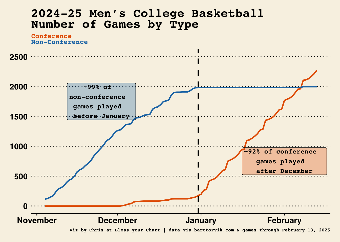
games_by_type <- games |> dplyr::distinct(game_id, .keep_all =TRUE) |> dplyr::group_by(date, type) |> dplyr::summarise(count = dplyr::n(), .groups ="drop") |> tidyr::complete(date =seq(min(date), max(date), by ="day"), type, fill =list(count =0)) |> dplyr::group_by(type) |> dplyr::arrange(date, .by_group =TRUE) |> dplyr::mutate(cumulative =cumsum(count)) |> dplyr::ungroup()type_plot <- games_by_type |> ggplot2::ggplot(ggplot2::aes(x = date, y = cumulative, color = type)) + ggplot2::geom_line(size =1) + ggplot2::scale_x_date(date_labels ="%B", date_breaks ="1 month") + ggplot2::scale_y_continuous(limits =c(0, 2500)) + ggplot2::labs(title ="2024-25 Men's College Basketball<br> Number of Games by Type", subtitle ="<span style='color: #e66101;'>Conference</span> <br> <span style='color: #1f78b4;'>Non-Conference</span>",caption ="Viz by Chris at Bless your Chart | data via barttorvik.com & games through February 13, 2025",x ="", y ="") + ggthemes::theme_wsj() + ggplot2::geom_vline(xintercept =as.Date("2024-12-31"), linetype ="dashed", color ="black", size =1) + ggplot2::scale_color_manual(values =c("#e66101", "#1f78b4")) + ggplot2::annotate("label",x =as.Date("2024-11-25"), y =1750,label ="~99% of \nnon-conference \ngames played \nbefore January", size =3.5, color ="black", fill ="#1f78b4",family ="mono",fontface ="bold",alpha = .3 ) + ggplot2::annotate("label",x =as.Date("2025-02-01"), y =750,label ="~92% of conference \ngames played \nafter December", size =3.5, color ="black", fill ="#e66101",family ="mono",fontface ="bold",alpha = .3 ) + ggplot2::theme(legend.position ="none",plot.title = ggtext::element_markdown(size =18,face ='bold',family ='mono' ),plot.subtitle = ggtext::element_markdown(size =10,family ='mono',face ='bold' ),plot.caption = ggtext::element_markdown(size =7, family ='mono', face ='bold') )ggplot2::ggsave("type_plot.png", type_plot,w =7.5,h =9,dpi =600,type ='cairo')type_plot
 Auburn
 Alabama
 Florida
 Tennessee
 Texas A&M
 Duke
Duke Houston
 Purdue
 Iowa St.
 Wisconsin
 Mississippi
 Memphis
 Michigan
 St. John’s
 Marquette
 Kentucky
 Kansas
 Arizona
 Texas Tech
 Michigan St.
 Louisville
 Mississippi St.
 Oregon