Call:
lm(formula = raw_em ~ tram, data = tram_data)

Residuals:
     Min       1Q   Median       3Q      Max
-18.9928  -4.9364  -0.1968   4.8903  23.4395

Coefficients:
            Estimate Std. Error t value Pr(>|t|)
(Intercept) -0.01631    0.38851  -0.042    0.967
tram         1.71733    0.08248  20.821   <2e-16 ***
---
Signif. codes:  0 '***' 0.001 '**' 0.01 '*' 0.05 '.' 0.1 ' ' 1

Residual standard error: 7.411 on 362 degrees of freedom
Multiple R-squared:  0.545, Adjusted R-squared:  0.5437
F-statistic: 433.5 on 1 and 362 DF,  p-value: < 2.2e-16
Code
r2_value <-summary(tram_raw)$r.squaredp_value <-summary(tram_raw)$coefficients[2,4]preds <-predict(tram_raw, newdata = tram_data)rmse_value <-sqrt(mean((tram_data$raw_em - preds)^2))# plot the residuals aug <- broom::augment(tram_raw, data = tram_data)highlight_teams <- aug |># use power conferences dplyr::filter(conf %in%c("ACC", "MW", "BE", "B12", "B10", "SEC")) |> dplyr::mutate(label =sprintf("%s\nActual Raw EM: %.1f\nPredicted: %.1f", team, raw_em, .fitted) ) |> dplyr::group_by(sign(.resid)) |> dplyr::slice_max(order_by =abs(.resid), n =50) |> dplyr::ungroup() |> dplyr::relocate(.fitted) |># arbitrary selection of a few interesting teams to highlight dplyr::filter(team %in%c("Seton Hall", "Oklahoma St.","Creighton", "Alabama"))
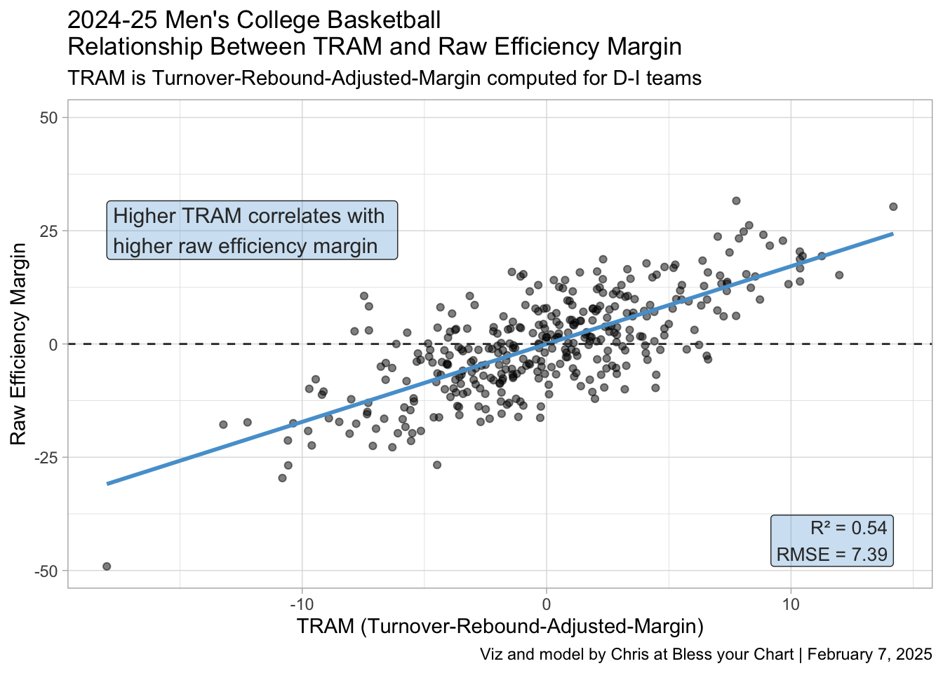
Team plot for TRAM model
Code
# limits for y-axismax_abs_y <-max(abs(tram_data$raw_em))team_plot <- tram_data |> ggplot2::ggplot(ggplot2::aes(x = tram, y = raw_em)) + ggplot2::geom_point(alpha =0.5) + ggplot2::geom_smooth(method ="lm", se =FALSE, color ="#56a0d3") + ggplot2::scale_y_continuous(limits =c(-max_abs_y, max_abs_y)) + ggplot2::geom_hline(yintercept =0, color ="#333333", linetype ="dashed") + ggplot2::labs(title ="2024-25 Men's College Basketball\nRelationship Between TRAM and Raw Efficiency Margin",subtitle ="TRAM is Turnover-Rebound-Adjusted-Margin computed for D-I teams",x ="TRAM (Turnover-Rebound-Adjusted-Margin)",y ="Raw Efficiency Margin", # Changed from "Raw EM"caption ="Viz and model by Chris at Bless your Chart | February 7, 2025" ) + ggplot2::theme_light() + ggplot2::annotate("label", x =max(tram_data$tram), y =min(tram_data$raw_em), label =sprintf("R² = %.2f\nRMSE = %.2f", r2_value, rmse_value),hjust =1, vjust =0, size =3.5, color ="#333333", fill ="#56a0d3",alpha = .3 ) + ggplot2::annotate("label", x =min(tram_data$tram), y =max(tram_data$raw_em),label ="Higher TRAM correlates with \nhigher raw efficiency margin", hjust =0, vjust =1, size =4, color ="#333333", fill ="#56a0d3",alpha = .3 )ggplot2::ggsave("team_plot.png", team_plot,w =9.5,h =7,dpi =600,type ='cairo')team_plot
Residual plot
Code
resid_plot <- aug |> ggplot2::ggplot(ggplot2::aes(x = tram, y = .resid)) + ggplot2::geom_point(alpha =0.3) + ggplot2::geom_hline(yintercept =0, linetype =2, color ="#acacac") + ggplot2::annotate("label", x =14, y =-15,label =paste("Highlighted Teams \nActual Raw EM, Predicted Raw EM \n",paste0(highlight_teams$team, " ( ", round(highlight_teams$raw_em, 1), ", ", round(highlight_teams$.fitted, 1), ")",collapse ="\n") ),hjust =1, vjust =0, color ="#333333", fill ="#56a0d3",alpha = .3, size =2.5, fontface ="bold" ) + cbbplotR::geom_cbb_teams(data = highlight_teams, ggplot2::aes(team = team),width = .03,position = ggplot2::position_dodge2(width =0.30, padding =0.15) ) + ggplot2::labs(title ="TRAM Model Residuals: Actual and Predicted Raw Efficiency",subtitle ="Positive residuals: team performs better than TRAM predicts\nNegative residuals: team performs worse than TRAM predicts",x ="TRAM (Turnover-Rebound-Adjusted-Margin)",y ="Residual (Actual - Predicted Raw Efficiency Margin)",caption ="Viz and model by Chris at Bless your Chart | February 7, 2025" ) + ggplot2::theme_light()ggplot2::ggsave("resid_plot.png", resid_plot,w =9.5,h =7,dpi =600,type ='cairo')resid_plot
Table for top TRAM teams
Code
tram_header <- glue::glue("<div style='display: flex; justify-content: space-between; align-items: center;'> <div> <img src='https://a.espncdn.com/combiner/i?img=/redesign/assets/img/icons/ESPN-icon-basketball.png' style='height: 40px; width: auto; vertical-align: middle;'> </div> <div style='flex-grow:1; margin-left: 30px; margin-right: 30px'> <span style='display: block; font-weight: bold; text-align: center; font-size: 24px;'>Teams with highest TRAM <br>Turnover-Rebound-Adjusted-Margin</span> <span style='font-size: 14px; font-weight: normal; display: block; text-align: center;'>Shows the teams with the highest TRAM along with the team's adjusted raw efficiency margin, raw efficiency margin, turnover and rebound rates for offense and defense.</span> </div> <div> <img src='https://a.espncdn.com/combiner/i?img=/redesign/assets/img/icons/ESPN-icon-basketball.png' style='height: 40px; width: auto; vertical-align: middle;'> </div> </div> <br>")team_tbl <- tram_data |> dplyr::filter(tram >9.5) |> dplyr::arrange(-tram) |> dplyr::select(team, tram, raw_em, adj_em, to_pct, or_pct, d_to_pct, d_or_pct) |> dplyr::mutate(tram =round(tram, 1)) |> cbbplotR::gt_cbb_teams(team, team) |> gt::gt() |> gtUtils::gt_theme_gtutils() |> gt::fmt_markdown(team) |> gt::cols_align(team, align ="left") |> gt::fmt(columns =c(tram, raw_em, adj_em),fns =function(x) {ifelse(x >0, paste0("+", x), x) } ) |> gt::cols_label(team ="",tram ="TRAM",raw_em ="Raw", adj_em ="Adjusted",to_pct ="TO%",or_pct ="OR%",d_to_pct ="TO%",d_or_pct ="DR%" ) |> gt::tab_header(title = gt::html(tram_header)) |> gt::tab_source_note(source_note = gt::html("<hr>These are teams that increase their efficiency through rebounds and turnovers. None of this data includes shooting performances.<hr>Data via hoopR and kenpom.com, theme via {gtUtils} and logos from ESPN.<hr><b>Table by Chris at Bless your chart | data through February 6 games</b>" ) ) |> gt::tab_spanner(label ="Offense", columns =c(to_pct, or_pct)) |> gt::tab_spanner(label ="Defense", columns =c(d_to_pct, d_or_pct)) |> gt::tab_spanner(label ="Efficiency Margin", columns =c(raw_em, adj_em)) |> gt::data_color(columns =c(tram, adj_em, raw_em),direction =c("column"),method =c("numeric"),palette ="Greens" ) |> gtUtils::gt_color_pills(to_pct,domain =c(.1, .20), format_type ="percent", digits =1,palette =c("#FFFACD", "#B0E57C") ) |> gtUtils::gt_color_pills(or_pct,domain =c(.25, .45), format_type ="percent", digits =1,palette =c("#FFFACD", "#B0E57C") ) |> gtUtils::gt_color_pills(d_to_pct,domain =c(.15, .25), format_type ="percent", digits =1,palette =c("#FFB6B6", "#D8BFD8"),reverse =TRUE ) |> gtUtils::gt_color_pills(d_or_pct,domain =c(.25, .33), format_type ="percent", digits =1,palette =c("#FFB6B6", "#D8BFD8"),reverse =TRUE ) |> gtUtils::gt_border_bars_bottom(c("#636363", "#969696", "#cccccc")) |> gt::tab_options(table.width = gt::px(675)) |> gtUtils::gt_border_grid(color ="black",weight =0.5,include_labels =FALSE) |> gtExtras::gt_add_divider(columns = team,sides ="right",color ="black") |> gt::tab_style(locations = gt::cells_source_notes(),style = gt::cell_text(font = gt::google_font("Signika Negative"),size = gt::px(11.5),weight =250 ) ) |> gt::tab_style(style =list(gt::cell_text(font = gt::google_font("Signika Negative"))),locations = gt::cells_body(columns =everything()) ) |> gt::tab_style(locations = gt::cells_column_spanners(),style = gt::cell_text(font = gt::google_font("Signika Negative"),weight =850,size = gt::px(15) ) ) gtUtils::gt_save_crop(team_tbl,file ="team_tbl.png",whitespace =60,bg ="#FFFDF5")team_tbl
Teams with highest TRAM
Turnover-Rebound-Adjusted-MarginShows the teams with the highest TRAM along with the team's adjusted raw efficiency margin, raw efficiency margin, turnover and rebound rates for offense and defense.
TRAM
Efficiency Margin
Offense
Defense
Raw
Adjusted
TO%
OR%
TO%
DR%
Houston
+14.2
+30.3
+34.8
14.3%
38.5%
22.5%
28.8%
Marquette
+12
+15.2
+23.7
12.9%
30.0%
23.7%
31.5%
St. John’s
+11.3
+19.4
+24.4
16.0%
37.5%
21.9%
28.1%
Iowa St.
+10.5
+19.4
+26.3
15.5%
33.8%
22.1%
27.8%
UCLA
+10.4
+16.7
+21.4
16.3%
32.2%
24.0%
29.2%
Texas A&M
+10.4
+13.8
+24.7
17.8%
42.8%
20.9%
28.1%
UC San Diego
+10.4
+18.7
+14.5
14.5%
26.7%
23.7%
27.2%
Saint Mary’s
+10.4
+20.4
+22.4
15.0%
40.9%
17.8%
25.9%
Vanderbilt
+9.9
+13.2
+15.1
14.4%
31.6%
22.1%
29.7%
Maryland
+9.7
+22.8
+24
14.8%
32.4%
20.8%
26.6%
These are teams that increase their efficiency through rebounds and turnovers. None of this data includes shooting performances.
Data via hoopR and kenpom.com, theme via {gtUtils} and logos from ESPN.
Table by Chris at Bless your chart | data through February 6 games

 Houston
 Marquette
 St. John’s
 Iowa St.
 UCLA
UCLA Texas A&M
 UC San Diego
 Saint Mary’s
 Vanderbilt
 Maryland