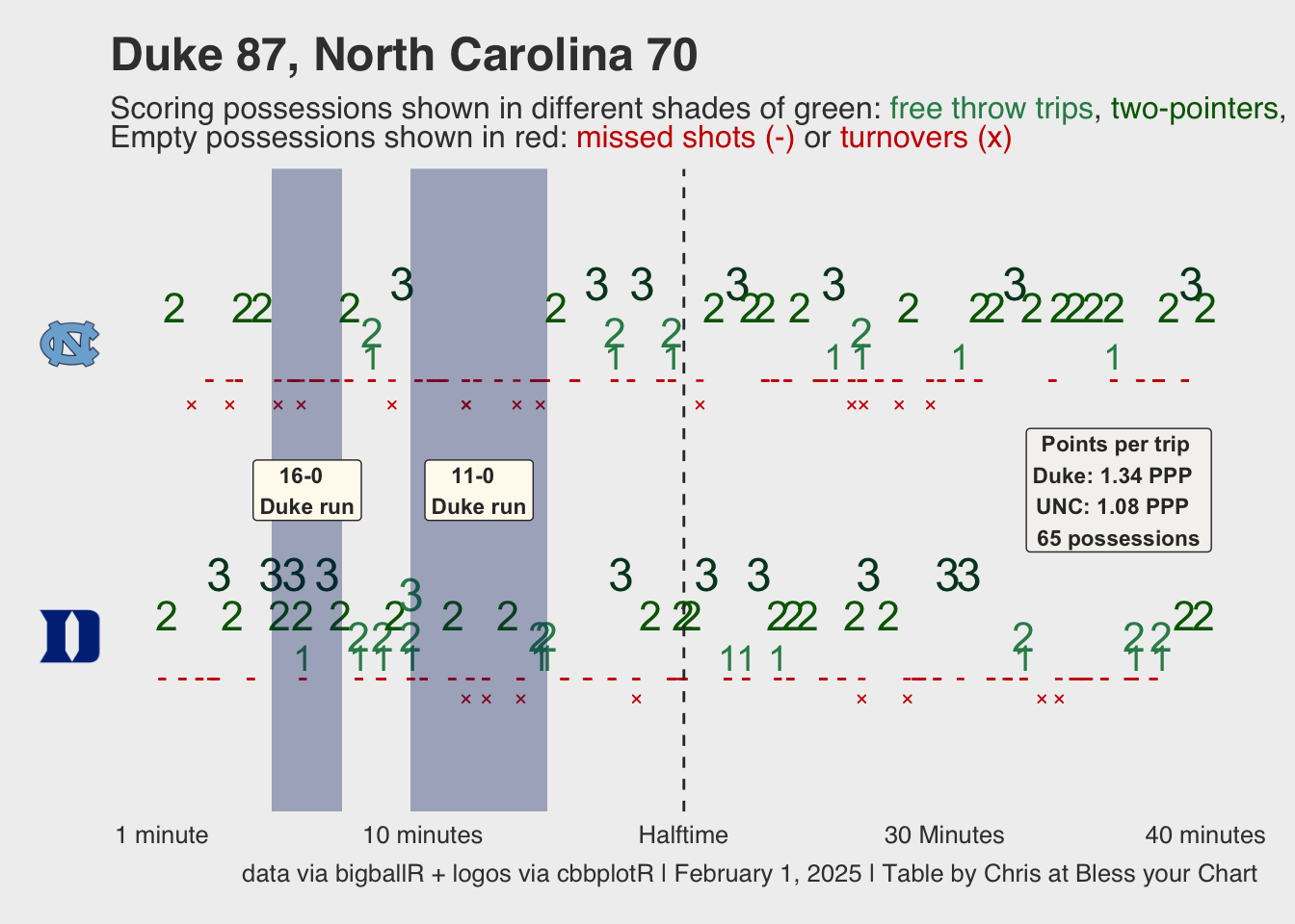
poss_plot <- game_plot |> ggplot2::ggplot(ggplot2::aes(x = Game_Seconds,y = Poss_Team,color = scoring_type,size = pts_value /2 )) + ggplot2::geom_point(ggplot2::aes(shape =factor(pts_shape)),position = ggplot2::position_dodge(width =0.5)) + ggplot2::scale_color_manual(values =c("free_throw"="#2E8B57", # Sea green for free throws"two_pointer"="#006400", # Dark green for 2-pointers"three_pointer"="#004225", # Deep forest green for 3-pointers"miss"="#cc0000", # Red for misses"turnover"="#cc0000"# Red for turnovers )) + ggplot2::scale_shape_manual(values =c(4, 45, 49, 50, 51)) + ggplot2::scale_x_continuous(breaks =c(0,600, 1200, 1800, 2400), labels =c("1 minute", "10 minutes", "Halftime", "30 Minutes", "40 minutes")) + ggplot2::geom_vline(xintercept =1200,linetype ="dashed",color ="#333333") + ggthemes::theme_fivethirtyeight() + ggplot2::annotate("rect",fill ="#012169",alpha =0.35,xmin =253,xmax =415,ymin =-Inf,ymax =Inf ) + ggplot2::annotate("rect",fill ="#012169",alpha =0.35,xmin =572,xmax =886,ymin =-Inf,ymax =Inf ) + ggplot2::theme(legend.position ="none",axis.text.y = cbbplotR::element_cbb_teams(size =0.9),panel.grid.major = ggplot2::element_blank(),panel.grid.minor = ggplot2::element_blank(),panel.background = ggplot2::element_blank(),plot.title = ggtext::element_markdown(),plot.subtitle = ggtext::element_markdown() ) + ggplot2::labs(x ="Possessions",y ="",title ="Duke 87, North Carolina 70",subtitle ="Scoring possessions shown in different shades of green: <span style='color:#2E8B57'>free throw trips</span>, <span style='color:#006400'>two-pointers</span>, <span style='color:#004225'>three-pointers</span><br>Empty possessions shown in red: <span style='color:#CC0000'>missed shots (-)</span> or <span style='color:#CC0000'>turnovers (x)</span>",caption ="data via bigballR + logos via cbbplotR | February 1, 2025 | Table by Chris at Bless your Chart" ) + ggplot2::annotate("label",x =2200,y =1.5,label ="Points per trip \nDuke: 1.34 PPP \nUNC: 1.08 PPP \n65 possessions",size =3,color ="#333333",fill ="floralwhite",fontface ="bold",alpha = .3 ) + ggplot2::annotate("label",x =334,y =1.5,label ="16-0 \nDuke run",size =3,color ="#333333",fill ="floralwhite",fontface ="bold" ) + ggplot2::annotate("label",x =729,y =1.5,label ="11-0 \nDuke run",size =3,color ="#333333",fill ="floralwhite",fontface ="bold" ) # save the plot ggplot2::ggsave("unc_duke_plot.png", poss_plot,w =9.5,h =7,dpi =600,type ='cairo')poss_plot
Load run data from bigballR
Code
# big assist from Connor over at https://github.com/cobrastats# commenting out all the code, and saving as a CSV to make the data static# schedule <- bigballR::get_team_schedule(team.name="North Carolina",season="2024-25")# pbp <- bigballR::get_play_by_play(schedule$Game_ID)# Filter for only made baskets# pbp <- pbp |># dplyr::filter(Shot_Value %in% c(1,2,3) & Event_Result=="made")# pbp <-pbp |># dplyr::group_by(ID) |># dplyr::arrange(Game_Seconds) |># dplyr::mutate(run = cumsum(Event_Team != lag(Event_Team, default = first(Event_Team))) + 1) |># dplyr::ungroup()# Calculate scoring runs# killshots <- pbp |># dplyr::group_by(ID,run) |># dplyr::summarise(run_team = first(Event_Team),# def_team = if_else(run_team==first(Home),first(Away),first(Home)),# run_length = sum(Shot_Value),# start_score = if_else(run_team==first(Home),paste0(first# (Home_Score)-first(Shot_Value),"-",first(Away_Score)),# paste0(first(Away_Score)-first(Shot_Value),"#-",first(Home_Score))),# end_score = if_else(run_team==first(Home),paste0(last(Home_Score# ),"-",last(Away_Score)),# paste0(last(Away_Score),"-",last(Home_Score3# ))),# run_start = paste0(first(Half_Status),"H-",first(Time)),# run_end = paste0(last(Half_Status),"H-",last(Time)),# time = last(Game_Seconds) - first(Game_Seconds),# time_clean = sprintf("%d:%02d", time %/% 60, time %% 60)# ) |># dplyr::arrange(desc(run_length)) |># dplyr::select(-run) |># dplyr::ungroup()run_data <- readr::read_csv("opp_runs.csv") |> dplyr::select(-1) |> dplyr::filter(run_team !="North Carolina") |> dplyr::select(run_team, run_length, start_score, end_score, run_start, run_end, time_clean) |> dplyr::filter(run_length >9) |> dplyr::mutate(time_clean =sub("^0?(\\d+):(\\d+):\\d+$", "\\1:\\2", time_clean))
Runs table
Code
run_header <- glue::glue("<div style='display: flex; justify-content: space-between; align-items: center;'> <div> <img src='https://a.espncdn.com/combiner/i?img=/i/teamlogos/ncaa/500/153.png' style='height: 45px; width: auto; vertical-align: middle;'> </div> <div style='flex-grow:1; margin-left: 30px; margin-right: 30px'> <span style='display: block; font-weight: bold; text-align: center; font-size: 24px;'>North Carolina <br>Opponent Scoring Runs of 10+ points</span> <span style='font-size: 14px; font-weight: normal; display: block; text-align: center;'>Shows scoring runs of 10+ points by opponent this season. <br>Carolina is 13-10 overall and 6-5 in the ACC through February 1 games.</span> </div> <div> <img src='https://a.espncdn.com/combiner/i?img=/redesign/assets/img/icons/ESPN-icon-basketball.png' style='height: 40px; width: auto; vertical-align: middle;'> </div> </div> <br>")run_tbl <- run_data |> cbbplotR::gt_cbb_teams(run_team, run_team) |> gt::gt() |> gtUtils::gt_theme_gtutils() |> gt::fmt_markdown(run_team) |> gt::fmt(columns =c(run_length),fns =function(x) {ifelse(x <0, paste0("+", x), x) } ) |> gtUtils::gt_column_subheaders(run_length =list(heading ="Run", subtitle ="# of points"),start_score =list(heading ="Start", subtitle ="Score"),end_score =list(heading ="End", subtitle ="Score"),run_start =list(heading ="Start", subtitle ="Time"),run_end =list(heading ="End", subtitle ="Time"),time_clean =list(heading ="Total", subtitle ="Time"),heading_color ="black",subtitle_color ="gray" ) |> gt::tab_header(title = gt::html(run_header)) |> gt::tab_source_note(source_note = gt::html("<hr>Score shows in perspective of opponent or the team making the run. The runs are also known as kill shots per Evan Miya.<hr>Data via bigballR + theme via {gtUtils} and logos from ESPN.<hr><b>Table by Chris at Bless your chart | data through February 1 games</b>" ) ) |> gt::tab_spanner(label ="Time", columns =c(run_start, run_end, time_clean)) |> gt::tab_spanner(label ="Score", columns =c(start_score, end_score)) |> gt::data_color(columns = run_length,direction =c("column"),method =c("numeric"),palette ="Reds" ) |> gtUtils::gt_border_bars_bottom(c("#56a0d3", "#89BDE0", "#BBD9ED")) |> gt::tab_options(table.width = gt::px(675)) |> gtUtils::gt_border_grid(color ="black",weight =0.5,include_labels =FALSE) |> gtExtras::gt_add_divider(columns = run_length,sides ="left",color ="black") |> gt::cols_label(run_team ="") |> gt::tab_style(locations = gt::cells_source_notes(),style = gt::cell_text(font = gt::google_font("Signika Negative"),size = gt::px(11.5),weight =250 ) ) |> gt::tab_style(style =list(gt::cell_text(font = gt::google_font("Signika Negative"))),locations = gt::cells_body(columns =everything()) ) |> gt::tab_style(locations = gt::cells_column_spanners(),style = gt::cell_text(font = gt::google_font("Signika Negative"),weight =850,size = gt::px(15) ) ) |> gt::cols_align(columns =c(run_team), align ="left") |> gtExtras::gt_highlight_rows( # this is silly rows =c(2, 4, 6),columns =c(run_team),fill ="#d0e4f3" ) |> gtExtras::gt_highlight_rows(rows =c(1, 3, 5, 7, 8, 9),columns =c(run_team),fill ="#ffe7e7" )gtUtils::gt_save_crop(run_tbl,file ="run_unc.png",whitespace =60,bg ="#FFFDF5")run_tbl
North Carolina
Opponent Scoring Runs of 10+ pointsShows scoring runs of 10+ points by opponent this season.
Carolina is 13-10 overall and 6-5 in the ACC through February 1 games.
Run # of points
Score
Time
Start Score
End Score
Start Time
End Time
Total Time
Duke
16
7-6
23-6
1H-15:47
1H-13:09
2:38
Elon
14
57-69
71-69
2H-10:43
2H-06:48
3:55
Louisville
12
70-69
82-69
2H-02:59
2H-00:40
2:19
Notre Dame
12
36-47
48-47
2H-15:46
2H-13:09
2:37
Wake Forest
12
37-39
49-39
2H-14:52
2H-09:36
5:16
Dayton
11
23-22
34-22
1H-07:47
1H-06:30
1:17
Duke
11
29-13
40-13
1H-10:27
1H-05:16
5:11
Florida
10
0-2
2-10
1H-17:32
1H-16:21
1:11
Kansas
10
39-29
49-29
1H-05:51
1H-01:43
4:08
Score shows in perspective of opponent or the team making the run. The runs are also known as kill shots per Evan Miya.
Data via bigballR + theme via {gtUtils} and logos from ESPN.
Table by Chris at Bless your chart | data through February 1 games

 Duke
Duke Elon
Elon Louisville
 Notre Dame
 Wake Forest
 Dayton
 Florida
 Kansas