custom_header <- glue::glue("<div style='display: flex; justify-content: space-between; align-items: center;'> <div> <img src='https://a.espncdn.com/combiner/i?img=/i/teamlogos/ncaa/500/153.png' style='height: 45px; width: auto; vertical-align: middle;'> </div> <div style='flex-grow:1; margin-left: 30px; margin-right: 30px'> <span style='display: block; font-weight: bold; text-align: center; font-size: 24px;'>North Carolina as a double-digit underdog against Duke</span> <span style='font-size: 12px; font-weight: normal; display: block; text-align: center;'>Since 1998, North Carolina is 9-5 against the spread with three outright wins as a double-digit underdog against Duke. The Blue Devils host UNC Saturday, and opened as a 13.5 point favorite per vegasinsider.com.</span> </div> <div> <img src='https://a.espncdn.com/combiner/i?img=/i/teamlogos/ncaa/500/150.png' style='height: 40px; width: auto; vertical-align: middle;'> </div> </div> <br>")duke_tbl <- duke_unc |> dplyr::select(date, location, spread, unc_cover, score, winner) |> gt::gt() |> gtUtils::gt_theme_gtutils() |> gtExtras::gt_merge_stack(col1 = date,col2 = location,palette =c("black", "#707070") ) |> gt::fmt_markdown(winner) |> gt::fmt_tf(columns = unc_cover,tf_style ="check-mark",colors =c("#56a0d3", "#003087"), ) |> gt::fmt(columns =c(spread),fns =function(x) {ifelse(x >0, paste0("+", x), x) } ) |> gtUtils::gt_column_subheaders(date =list(heading ="Date", subtitle ="Location"),winner =list(heading ="Winner", subtitle ="Outright"),score =list(heading ="Score", subtitle ="Final"),spread =list(heading ="Spread", subtitle ="UNC as Underdog"),unc_cover =list(heading ="Cover?", subtitle ="UNC"),heading_color ="black",subtitle_color ="gray" ) |> gt::tab_header(title = gt::html(custom_header)) |> gt::tab_source_note(source_note = gt::html("<hr>Data via TeamRankings.com's BetIQ tool, theme via {gtUtils} and logos from ESPN.<hr><b>Table by Chris at Bless your chart</b>" ) ) |> gtUtils::gt_border_bars_bottom(c("#56a0d3", "#89BDE0", "#BBD9ED")) |> gt::tab_options(table.width = gt::px(550)) |> gtUtils::gt_border_grid(color ="black",weight =1,include_labels =FALSE) |> gt::tab_style(locations = gt::cells_source_notes(),style = gt::cell_text(font = gt::google_font("Signika Negative"),size = gt::px(11.5),weight =250 ) ) |> gt::tab_style(style =list(gt::cell_text(font = gt::google_font("Signika Negative"))),locations = gt::cells_body(columns =everything()) ) |> gt::cols_align(columns =c(winner, spread), align ="right") |> gt::cols_align(columns =c(date, score, unc_cover), align ="left") |> gtExtras::gt_highlight_rows(rows =c(8, 13, 14), fill ="#d0e4f3") |> gt::tab_style(style =list(gt::cell_text(font = gt::google_font("Signika Negative"),color ="#003087" )),locations = gt::cells_body(columns =c(score), rows =c(1:7, 9:11)) ) |> gt::tab_style(style =list(gt::cell_text(font = gt::google_font("Signika Negative"),color ="#56a0d3" )),locations = gt::cells_body(columns =c(spread)))gtUtils::gt_save_crop(duke_tbl,file ="duke_unc.png",whitespace =60,bg ="#FFFDF5")duke_tbl
North Carolina as a double-digit underdog against DukeSince 1998, North Carolina is 9-5 against the spread with three outright wins as a double-digit underdog against Duke. The Blue Devils host UNC Saturday, and opened as a 13.5 point favorite per vegasinsider.com.
Date Location
Spread UNC as Underdog
Cover? UNC
Score Final
Winner Outright
March 03, 2002
Cameron Indoor Stadium
+28
✔
Duke 93, UNC 68
March 08, 2002
Charlotte Coliseum
+26
✔
Duke 60, UNC 48
January 31, 2002
Dean E. Smith Center
+17
✘
Duke 87, UNC 58
January 27, 1999
Cameron Indoor Stadium
+16
✔
Duke 89, UNC 77
March 06, 2010
Cameron Indoor Stadium
+15
✘
Duke 82, UNC 50
February 05, 2003
Cameron Indoor Stadium
+14
✔
Duke 83, UNC 74
March 07, 1999
Charlotte Coliseum
+12
✘
Duke 96, UNC 73
March 05, 2022
Cameron Indoor Stadium
+11
✔
UNC 94, Duke 81
March 04, 2000
Cameron Indoor Stadium
+11
✘
Duke 90, UNC 76
March 07, 2020
Cameron Indoor Stadium
+10.5
✘
Duke 89, UNC 76
February 13, 2013
Cameron Indoor Stadium
+10.5
✔
Duke 73, UNC 68
February 09, 2011
Cameron Indoor Stadium
+10.5
✔
Duke 79, UNC 73
February 01, 2001
Cameron Indoor Stadium
+10.5
✔
UNC 85, Duke 83
February 20, 2019
Cameron Indoor Stadium
+10
✔
UNC 88, Duke 72
Data via TeamRankings.com's BetIQ tool, theme via {gtUtils} and logos from ESPN.
Table by Chris at Bless your chart
North Carolina: Scoring Spurts by OpponentShows scoring runs of 6+ points or more in a given game.
Carolina is 13-9 overall and 6-4 in the ACC through January 28 games.
Opponent Spurts
+/- From Runs
UNC Spurts
# 6+ points
Avg Points
Total From spurts
# 6+ points
Avg Points
Total From spurts
UCLA
5
7.6
38
-6
4
8.0
32
Florida
5
7.4
37
-15
2
11.0
22
Kansas
4
8.0
32
-16
2
8.0
16
Pittsburgh
4
7.8
31
-6
4
6.2
25
Wake Forest
4
7.8
31
-6
4
6.2
25
Auburn
4
7.5
30
+1
4
7.8
31
Michigan St.
4
7.5
30
-17
2
6.5
13
Elon
3
9.0
27
+21
6
8.0
48
SMU
4
6.2
25
+11
5
7.2
36
Hawaii
4
6.0
24
+9
4
8.2
33
Notre Dame
3
8.0
24
-4
3
6.7
20
North Carolina St.
3
7.0
21
-5
2
8.0
16
Louisville
2
9.5
19
-11
1
8.0
8
Alabama
2
7.5
15
+18
5
6.6
33
Campbell
2
6.0
12
+29
6
6.8
41
Dayton
1
11.0
11
+3
2
7.0
14
Boston College
1
6.0
6
+27
5
6.6
33
Georgia Tech
1
6.0
6
+7
1
13.0
13
La Salle
1
6.0
6
+39
5
9.0
45
Stanford
1
6.0
6
+6
2
6.0
12
American
0
0.0
0
+70
9
7.8
70
California
0
0.0
0
+22
2
11.0
22
Data via bigballR + theme via {gtUtils} and logos from ESPN.
Table by Chris at Bless your chart | data through January 28 games
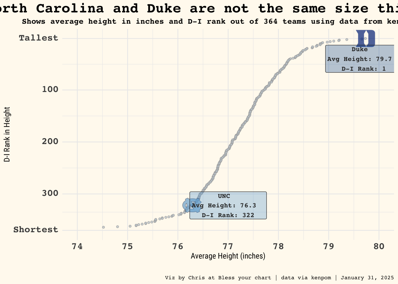
Height table
Code
# pull CSVs down from kenpom # could do this via hoopR, but just grabbed CSVs because I want to look at data first# duke_ht <- summary25_1_ |> # dplyr::left_join(height25, by = "TeamName") |> # dplyr::select(team = TeamName, # adjem = AdjEM, # size = Size,# sizerk = SizeRank)# save as csv # write.csv(duke_ht, "duke_ht.csv")# load dataduke_ht <- readr::read_csv("duke_ht.csv")# add theme theme_me <-function() {# Create a base theme with minimal style base_theme <- ggplot2::theme_minimal(base_size =10, base_family ="RobotoCondensed-Regular")# Customize the base theme with additional modifications custom_theme <- base_theme + ggplot2::theme(plot.title = ggplot2::element_text(hjust =0.5,size =24,face ="bold" ),plot.subtitle = ggplot2::element_text(hjust =0.5,size =10,lineheight =0.25,vjust =-0.5 ),plot.caption = ggplot2::element_text(hjust =1,size =6,lineheight =0.35,margin = ggplot2::margin(t =20) ),plot.background = ggplot2::element_rect(fill ="floralwhite", color ="floralwhite") )return(custom_theme)}# make the plotduke_is_tall <- duke_ht |> ggplot2::ggplot(ggplot2::aes(x = size, y = sizerk)) + ggplot2::geom_point(color ="#acacac",fill ="#c4ced4",shape =21,size =1,alpha = .75 ) + ggplot2::scale_x_continuous(limits =c(74, 80), breaks =seq(74, 80, 1)) + ggplot2::scale_y_reverse(limits =c(370, 1),breaks =c(370, 300, 200, 100, 1),labels =c("Shortest", "300", "200", "100", "Tallest") ) + ggplot2::annotate( cfbplotR::GeomCFBlogo,x =76.28,y =322,team ="North Carolina",height = .10,alpha = .7 ) + ggplot2::annotate( cfbplotR::GeomCFBlogo,x =79.73,y =1,team ="Duke",height = .10,alpha = .7 ) +theme_me() + ggplot2::theme(plot.title = ggtext::element_markdown(size =18,face ='bold',family ='mono' ),plot.subtitle = ggtext::element_markdown(size =10,family ="mono",face ="bold" ),plot.caption = ggtext::element_markdown(size =7, family ='mono'),axis.text.x = ggtext::element_markdown(size =12,family ='mono',face ='bold' ),axis.text.y = ggtext::element_markdown(size =12,family ='mono',face ='bold' ) ) + ggplot2::labs(x ="Average Height (inches)",y ="D-I Rank in Height",title ="North Carolina and Duke are not the same size this season",subtitle ="Shows average height in inches and D-I rank out of 364 teams using data from kenpom.com",caption ="Viz by Chris at Bless your chart | data via kenpom | January 31, 2025" ) + ggplot2::annotate(geom ="label",x =77,y =322,label ="UNC \nAvg Height: 76.3 \nD-I Rank: 322",fill ="#56a0d3",color ="#333333",size =3,fontface ='bold',family ='mono',alpha = .3,hjust =0.5 ) + ggplot2::annotate(geom ="label",x =79.7,y =40,label ="Duke \nAvg Height: 79.7 \nD-I Rank: 1",fill ="#00539B",color ="#333333",size =3,fontface ='bold',family ='mono',alpha = .3,hjust =0.5 )# save plotggplot2::ggsave("duke_is_tall_plot.png", duke_is_tall,w =10.5,h =8.5,dpi =600,bg ="white",type ='cairo')duke_is_tall
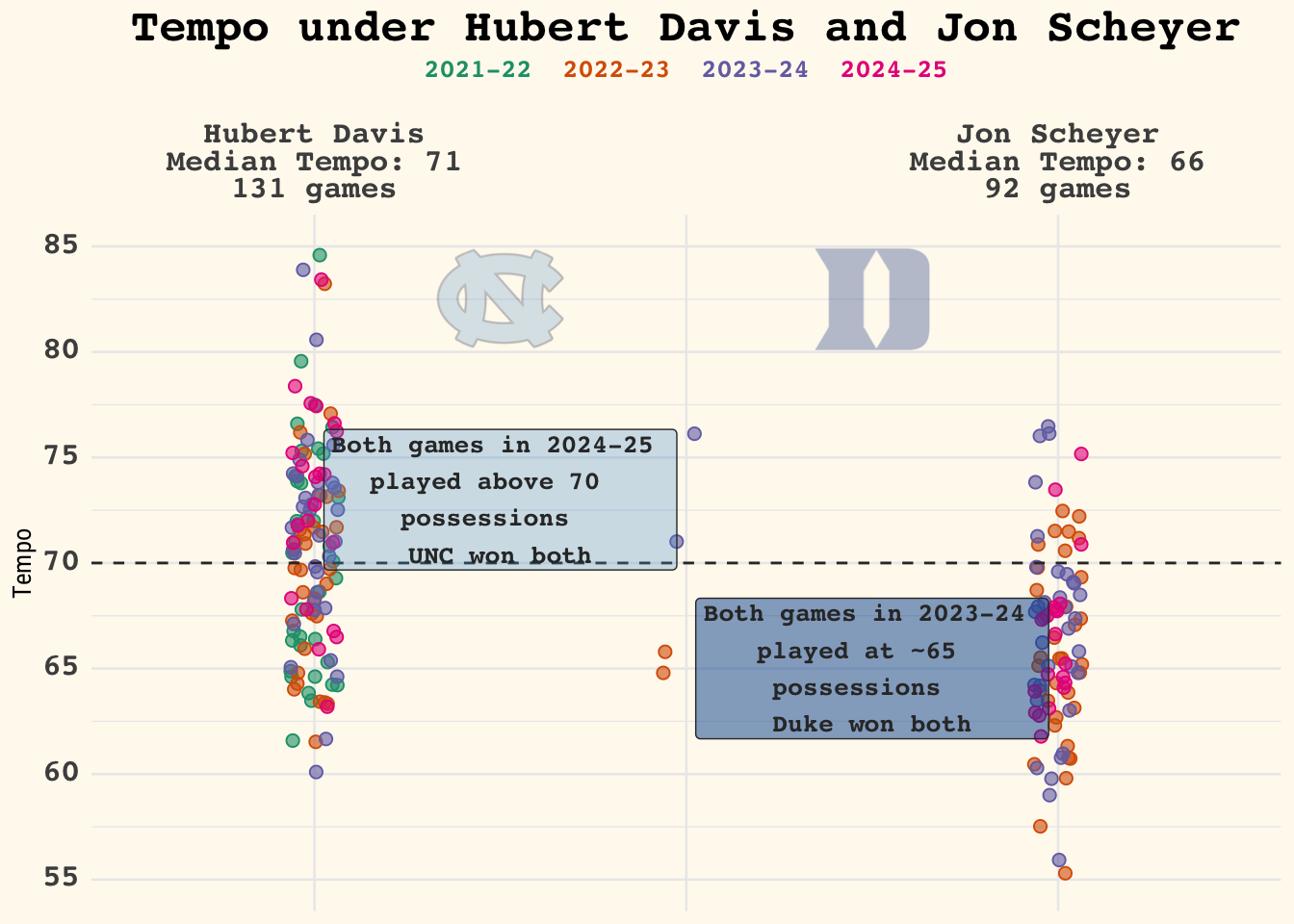
Tempo plot
Code
# this is a refresh of an old plot, see previous code here:# https://cjg.quarto.pub/bless-your-chart/posts/byc_074/byc_074_davis_schyer.html# saved the data as a CSV to make it easier to pull staticallyunc_duke_tempo <- readr::read_csv("unc_duke_tempo.csv")my_fill <- ggplot2::aes(fill = ggplot2::after_scale(ggplot2::alpha(colour, 0.6)))theme_me <-function() {# Create a base theme with minimal style base_theme <- ggplot2::theme_minimal(base_size =10, base_family ="RobotoCondensed-Regular")# Customize the base theme with additional modifications custom_theme <- base_theme + ggplot2::theme(plot.title = ggplot2::element_text(hjust =0.5,size =24,face ="bold" ),plot.subtitle = ggplot2::element_text(hjust =0.5,size =10,lineheight =0.25,vjust =-0.5 ),plot.caption = ggplot2::element_text(hjust =1,size =6,lineheight =0.35,margin = ggplot2::margin(t =20) ),plot.background = ggplot2::element_rect(fill ="floralwhite", color ="floralwhite") )return(custom_theme)}# combine the datasetstempo_plot <- unc_duke_tempo |> ggplot2::ggplot(ggplot2::aes(x = coach, y = tempo)) + ggplot2::geom_jitter(shape =21,width = .065,size =2, ggplot2::aes(colour =factor(year), !!!my_fill) ) +theme_me() + ggplot2::labs(x ="",y ="Tempo",title ="Tempo under Hubert Davis and Jon Scheyer",subtitle ="<span style='color: #1b9e77;'>2021-22</span> <span style='color: #d95f02;'>2022-23</span> <span style='color: #7570b3;'>2023-24</span> <span style='color: #e7298a;'>2024-25</span>","Viz by Chris at Bless your chart | data via kenpom | January 31, 2025" ) + ggplot2::scale_x_discrete(position ="top",labels =c("Hubert Davis \nMedian Tempo: 71 \n131 games","","Jon Scheyer \nMedian Tempo: 66 \n92 games" ) ) + ggplot2::scale_y_continuous(limits =c(55, 85), breaks =seq(55, 85, 5)) + ggplot2::scale_color_manual(values =c("#1b9e77", "#d95f02", "#7570b3", "#e7298a")) + ggplot2::geom_hline(yintercept =70,linetype ="dashed",color ="#333333") + ggplot2::theme(legend.position ="none",plot.title = ggtext::element_markdown(size =18,face ='bold',family ='mono' ),strip.text.x = ggtext::element_markdown(size =12,face ='bold',family ='mono' ),plot.subtitle = ggtext::element_markdown(size =10,family ="mono",face ="bold" ),plot.caption = ggtext::element_markdown(size =7, family ='mono'),axis.text.x = ggtext::element_markdown(size =12,family ='mono',face ='bold' ),axis.text.y = ggtext::element_markdown(size =12,family ='mono',face ='bold' ) ) + ggplot2::annotate("label",x =2.5,y =65,label ="Both games in 2023-24 \nplayed at ~65 \npossessions \nDuke won both",size =3.5,color ="#333333",fill ="#00539B",family ="mono",fontface ="bold",alpha = .5 ) + ggplot2::annotate("label",x =1.5,y =73,label ="Both games in 2024-25 \nplayed above 70 \npossessions \nUNC won both",size =3.5,color ="#333333",fill ="#56a0d3",family ="mono",fontface ="bold",alpha = .3 ) + ggplot2::annotate( cfbplotR::GeomCFBlogo,x =2.5,y =82.5,team ="Duke",height = .18,alpha = .3 ) + ggplot2::annotate( cfbplotR::GeomCFBlogo,x =1.5,y =82.5,team ="North Carolina",height = .20,alpha = .3 )ggplot2::ggsave("scheyer_davis.png", tempo_plot,w =8,h =10.5,dpi =600,type ='cairo')tempo_plot


 UCLA
UCLA Florida
 Kansas
 Pittsburgh
 Wake Forest
 Auburn
 Michigan St.
 Elon
Elon SMU
SMU Hawaii
 Notre Dame
 North Carolina St.
 Louisville
 Alabama
 Campbell
 Dayton
 Boston College
 Georgia Tech
 La Salle
 Stanford
 American
 California