098: NBA Draft

Load and manipulate data

nbadraft <- readr::read_csv("nba_draft_04.csv")

# cover years where a team had no picks
all_years <- seq(min(nbadraft$`Draft Year`), max(nbadraft$`Draft Year`))

# manipulate data to count picks over time 
lotdraft <- nbadraft |> 
  dplyr::group_by(`Draft Year`, College) |> 
  dplyr::summarise(picks = dplyr::n(), .groups = 'drop') |> 
  tidyr::complete(`Draft Year` = all_years, College, fill = list(picks = 0)) |> 
  dplyr::arrange(College, `Draft Year`) |> 
  dplyr::group_by(College) |> 
  dplyr::mutate(all_lot_picks = cumsum(picks)) |> 
  dplyr::ungroup() |> 
  dplyr::mutate(College = dplyr::if_else(is.na(College), "No College", College)) |> 
  dplyr::arrange(`Draft Year`)

Make line chart of picks over time

lotdraft |> 
  ggplot2::ggplot(ggplot2::aes(x = `Draft Year`, y = all_lot_picks, color = College)) +
  ggplot2::geom_line(linewidth = 0.5) +
  ggplot2::geom_hline(yintercept = 10, linetype = "dashed", color = "#333333") +
  ggplot2::geom_vline(xintercept = 2006, linetype = "dashed", color = "#333333") +
  ggplot2::geom_line(data = lotdraft |> dplyr::filter(College %in% c("No College",
                                                                     "Kentucky",
                                                                     "Duke",
                                                                     "Connecticut",
                                                                     "Kansas",
                                                                     "North Carolina",
                                                                     "Arizona")), 
                     linewidth = 1.5) +
  ggplot2::scale_color_manual(values = c("No College" = "#d01c8b",
                                         "Kentucky" = "#0033A0",
                                         "Duke" = "#003087",
                                         "Kansas" = "#0051BA",
                                         "Connecticut" = "#000E2F",
                                         "North Carolina" = "#56a0d3",
                                         "Arizona" = "#CC0033",
                                         Other = "#eeeeee")) +
  ggplot2::scale_x_continuous(breaks = seq(2004, 2023, 1)) +
  ggplot2::scale_y_continuous(breaks = seq(0, 50, 5), limits = c(0, 50)) +
  ggplot2::annotate(
    geom = "label",
    x = 2023.8,
    y = 42.5,
    color = "#333333",
    fill = "#d01c8b",
    label = "No \nCollege",
    size = 4,
    fontface = 'bold',
    family = 'mono',
    alpha = 0.3
  ) +
  ggplot2::annotate(
    geom = "label",
    x = 2023.8,
    y = 5,
    color = "#333333",
    fill = "#acacac",
    label = "Other \nColleges",
    size = 3.5,
    fontface = 'bold',
    family = 'mono',
    alpha = 0.3
  ) +
  ggplot2::annotate(
    geom = "curve",
    color = "#d01c8b",
    x = 2011.5,
    y = 32,
    xend = 2021.5,
    yend = 38.5,
    curvature = -.3,
    linewidth = 1.3,
    arrow = ggplot2::arrow(length = ggplot2::unit(4, "mm"))
  ) +
  ggplot2::annotate(
    geom = "label",
    x = 2011.2,
    y = 28.9,
    color = "#333333",
    fill = "#d01c8b",
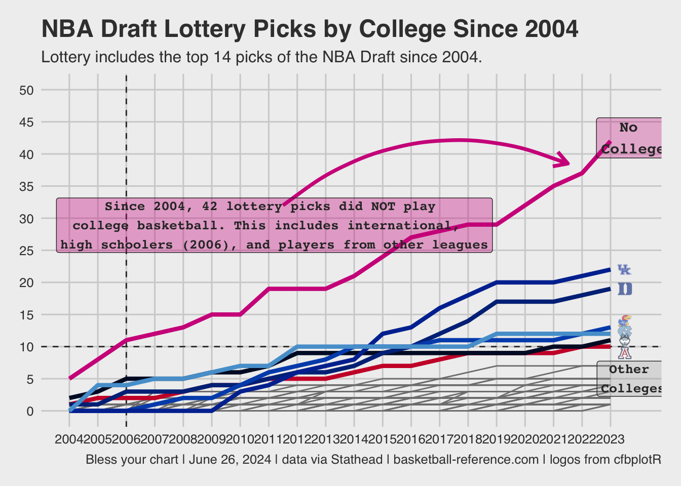
    label = "Since 2004, 42 lottery picks did NOT play \ncollege basketball. This includes international,  \nhigh schoolers (2006), and players from other leagues",
    size = 3.5,
    fontface = 'bold',
    family = 'mono',
    alpha = 0.35
  ) +
  ggplot2::annotate(
    cfbplotR::GeomCFBlogo,
    x = 2023.5,
    y = 22,
    team = "Kentucky",
    height = .045,
    alpha = 0.6
  ) +
  ggplot2::annotate(
    cfbplotR::GeomCFBlogo,
    x = 2023.5,
    y = 19,
    team = "Duke",
    height = .045,
    alpha = 0.6
  ) +
  ggplot2::annotate(
    cfbplotR::GeomCFBlogo,
    x = 2023.5,
    y = 14,
    team = "Kansas",
    height = .045,
    alpha = 0.6
  ) +
  ggplot2::annotate(
    cfbplotR::GeomCFBlogo,
    x = 2023.5,
    y =12.4,
    team = "North Carolina",
    height = .045,
    alpha = 0.6
  ) +
  ggplot2::annotate(
    cfbplotR::GeomCFBlogo,
    x = 2023.5,
    y = 11,
    team = "Connecticut",
    height = .045,
    alpha = 0.6
  ) +
  ggplot2::annotate(
    cfbplotR::GeomCFBlogo,
    x = 2023.5,
    y = 9,
    team = "Arizona",
    height = .045,
    alpha = 0.6
  ) +
  ggthemes::theme_fivethirtyeight() +
  ggplot2::theme(legend.position = "none") + 
  ggplot2::labs(
    title = "NBA Draft Lottery Picks by College Since 2004",
    subtitle = "Lottery includes the top 14 picks of the NBA Draft since 2004.",
    caption = "Bless your chart | June 26, 2024 | data via Stathead | basketball-reference.com | logos from cfbplotR",
    x = "Year",
    y = "Draft Picks"
  ) -> nba_lot_plot 

ggplot2::ggsave(
  "nba_lot_plot.png",
  nba_lot_plot,
  w = 11.5,
  h = 7.9,
  dpi = 600,
  type = 'cairo'
)

nba_lot_plot