089: Coach Changes

Load data

cbbdata::cbd_torvik_game_factors() |>
  dplyr::filter(year > 2018) |>
  dplyr::group_by(team) |>
  dplyr::summarise(unique_coaches = dplyr::n_distinct(coach)) |>
  dplyr::arrange(-unique_coaches) -> coach_change

thisyr_teams <- readr::read_csv("teams.csv")

coach_change |> 
  dplyr::left_join(thisyr_teams, by = "team") |> 
  dplyr::mutate(total = tidyr::replace_na(total, 0)) |> 
  dplyr::mutate(changes = unique_coaches + total) -> full_changes

Coach bar plot

theme_me <- function() {
  # Create a base theme with minimal style
  base_theme <- ggplot2::theme_minimal(base_size = 10, base_family = "RobotoCondensed-Regular")
  
  # Customize the base theme with additional modifications
  custom_theme <- base_theme +
    ggplot2::theme(
      plot.title = ggplot2::element_text(
        hjust = 0.5,
        size = 24,
        face = "bold"
      ),
      plot.subtitle = ggplot2::element_text(
        hjust = 0.5,
        size = 10,
        lineheight = 0.25,
        vjust = -0.5
      ),
      plot.caption = ggplot2::element_text(
        hjust = 1,
        size = 6,
        lineheight = 0.35,
        margin = ggplot2::margin(t = 20)
      ),
      plot.background = ggplot2::element_rect(fill = "floralwhite", color = "floralwhite")
    )
  
  return(custom_theme)
} 


full_changes |> 
  dplyr::group_by(changes) |> 
  dplyr::summarise(count = dplyr::n()) |> 
  ggplot2::ggplot(ggplot2::aes(x = changes, y = count, fill = as.factor(changes))) +
  ggplot2::geom_bar(stat = "identity") +
  ggplot2::scale_fill_brewer(palette = "Set2") +
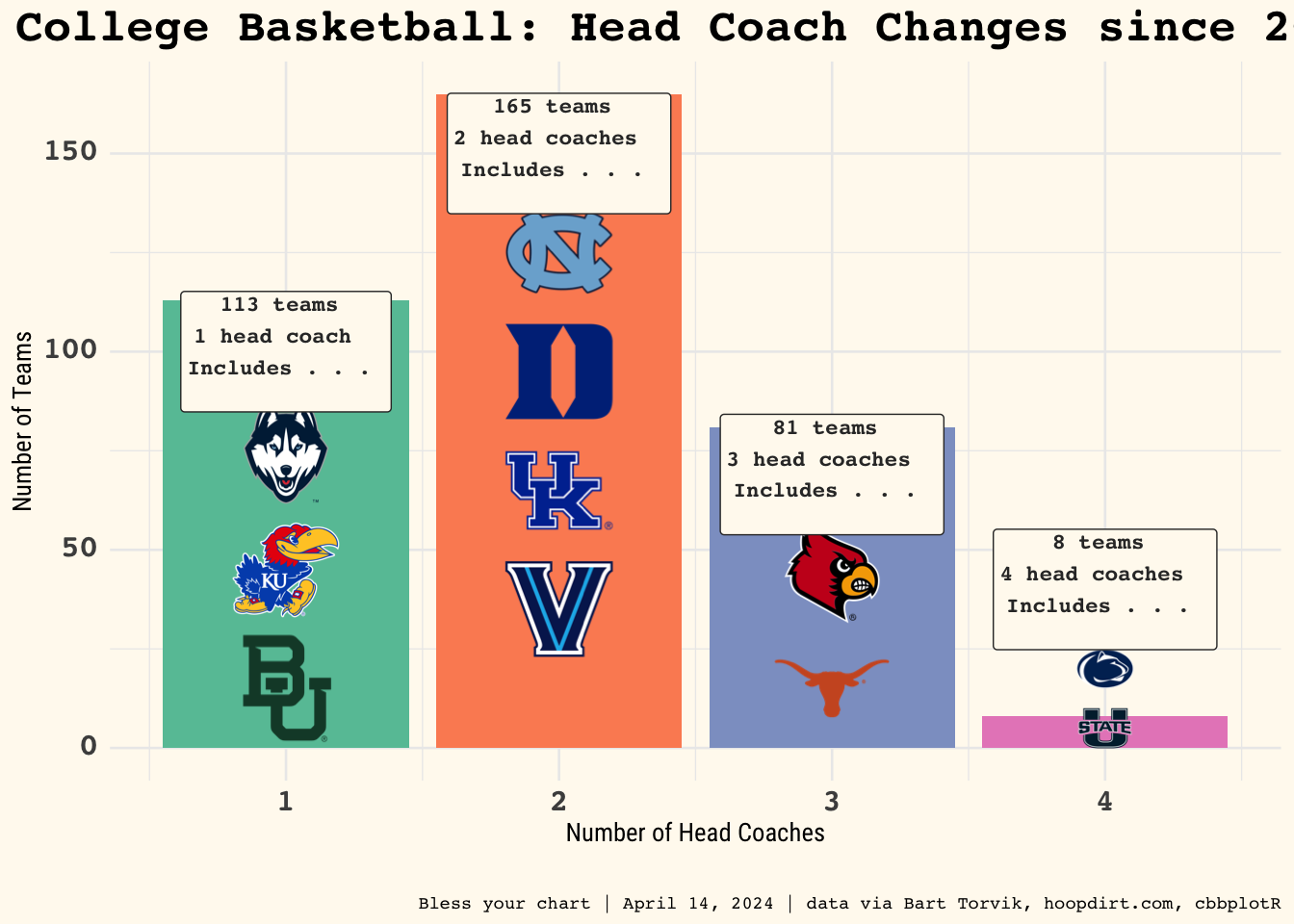
  ggplot2::labs(title = "College Basketball: Head Coach Changes since 2019",
       x = "Number of Head Coaches",
       y = "Number of Teams",
       caption = "Bless your chart | April 14, 2024 | data via Bart Torvik, hoopdirt.com, cbbplotR") +
  theme_me() +
  ggplot2::theme(legend.position = "none",
                 plot.title = ggtext::element_markdown(size = 18, face ='bold', family = 'mono'),
                 strip.text.x = ggtext::element_markdown(size = 12, 
                                                         face ='bold', family = 'mono'),
                 plot.subtitle = ggtext::element_markdown(size = 10, family = "mono", face = "bold"),
                 plot.caption = ggtext::element_markdown(size = 7, family = 'mono'),
                 axis.text.x = ggtext::element_markdown(size = 12, family = 'mono', face ='bold'),  
                 axis.text.y = ggtext::element_markdown(size = 12, family = 'mono', face ='bold')
  ) +
  ggplot2::annotate(cfbplotR::GeomCFBlogo,
                    x = 1, 
                    y = 75, 
                    team = "Connecticut",
                    width = .10) +
  ggplot2::annotate(cfbplotR::GeomCFBlogo,
                    x = 1, 
                    y = 45, 
                    team = "Kansas",
                    width = .10) +
  ggplot2::annotate(cfbplotR::GeomCFBlogo,
                    x = 1, 
                    y = 15, 
                    team = "Baylor",
                    width = .10) +
  ggplot2::annotate(cfbplotR::GeomCFBlogo,
                    x = 2, 
                    y = 125, 
                    team = "North Carolina",
                    width = .10) +
  ggplot2::annotate(cfbplotR::GeomCFBlogo,
                    x = 2, 
                    y = 95, 
                    team = "Duke",
                    width = .10) +
  ggplot2::annotate(cfbplotR::GeomCFBlogo,
                    x = 2, 
                    y = 65, 
                    team = "Kentucky",
                    width = .10) +
  ggplot2::annotate(cfbplotR::GeomCFBlogo,
                    x = 2, 
                    y = 35, 
                    team = "Villanova",
                    width = .10) +
  ggplot2::annotate(cfbplotR::GeomCFBlogo,
                    x = 3, 
                    y = 45, 
                    team = "Louisville",
                    width = .10) +
  ggplot2::annotate(cfbplotR::GeomCFBlogo,
                    x = 3, 
                    y = 15, 
                    team = "Texas",
                    width = .10) +
  ggplot2::annotate(cfbplotR::GeomCFBlogo,
                    x = 4, 
                    y = 20, 
                    team = "Penn State",
                    width = .05) +
  ggplot2::annotate(cfbplotR::GeomCFBlogo,
                    x = 4, 
                    y = 5, 
                    team = "Utah State",
                    width = .05) +
  ggplot2::annotate(
    "label",
    x = 1,
    y = 100,
    label = "113 teams \n1 head coach  \nIncludes . . . \n",
    size = 3,
    color = "#333333",
    fill = "floralwhite",
    family = "mono",
    fontface = "bold"
  ) +
  ggplot2::annotate(
    "label",
    x = 2,
    y = 150,
    label = "165 teams \n2 head coaches  \nIncludes . . . \n",
    size = 3,
    color = "#333333",
    fill = "floralwhite",
    family = "mono",
    fontface = "bold"
  ) +
  ggplot2::annotate(
    "label",
    x = 3,
    y = 69,
    label = "81 teams \n3 head coaches  \nIncludes . . . \n",
    size = 3,
    color = "#333333",
    fill = "floralwhite",
    family = "mono",
    fontface = "bold"
  ) +
  ggplot2::annotate(
    "label",
    x = 4,
    y = 40,
    label = "8 teams \n4 head coaches  \nIncludes . . . \n",
    size = 3,
    color = "#333333",
    fill = "floralwhite",
    family = "mono",
    fontface = "bold"
  ) -> coach_plot
  
  ggplot2::ggsave(
    "coach_plot.png",
    coach_plot,
    w = 8.5,
    h = 8.5,
    dpi = 600,
    type = 'cairo'
  )

  coach_plot