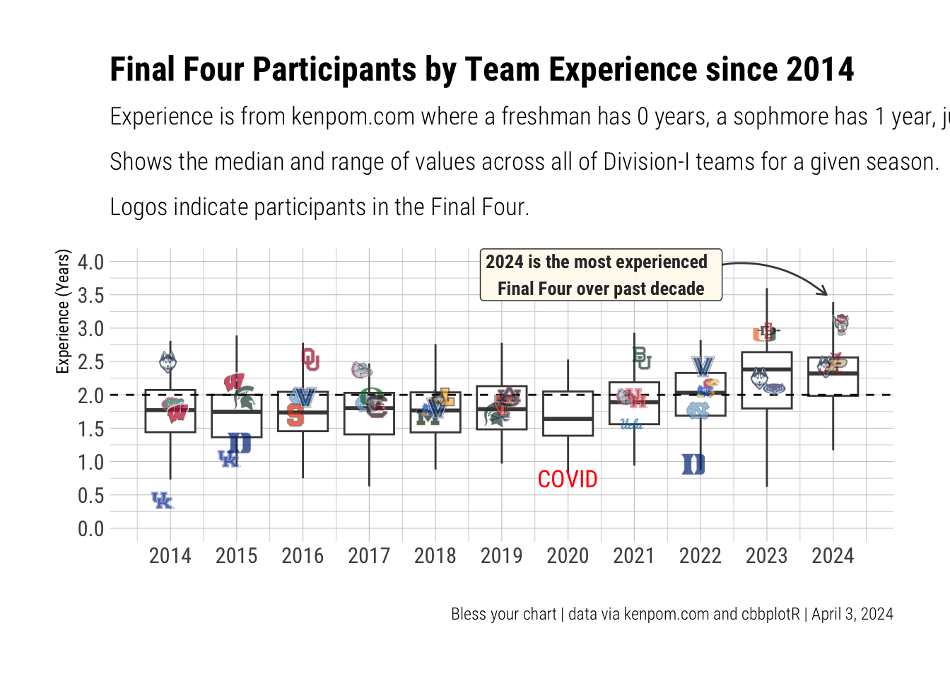
088: Experience

Load data

library(cbbplotR)
yrs <- c(2008:2024)

rm <- function(id) {
  hoopR::kp_height(min_year = id, max_year = id) |>  
    dplyr::mutate(season = id) |> 
    dplyr::select(season, ncaa_seed, team, continuity, 
                  continuity_rk, bench, bench_rk, experience, experience_rk) |> 
    dplyr::filter(!is.na(ncaa_seed))
}


rm_data <- lapply(yrs, rm)

rm_results <- as.data.frame(do.call(rbind, rm_data))

# final four
finalfours <- tibble::tribble(
  ~season,~team,~result,
  2008,"Memphis","F4",
  2008,"Kansas","Champs",
  2008,"North Carolina","F4",
  2008,"UCLA","F4",
  2009,"North Carolina","Champs",
  2009,"Michigan St.","F4",
  2009,"Connecticut","F4",
  2009,"Villanova","F4",
  2010,"Butler","F4",
  2010,"Duke","Champs",
  2010,"West Virginia","F4",
  2010,"Michigan St.","F4",
  2011,"Butler","F4",
  2011,"Connecticut","Champs",
  2011,"Kentucky","F4",
  2011,"VCU","F4",
  2012,"Kansas","F4",
  2012,"Kentucky","Champs",
  2012,"Louisville","F4",
  2012,"Ohio St.","F4",
  2013,"Michigan","F4",
  2013,"Louisville","Champs",
  2013,"Syracuse","F4",
  2013,"Wichita St.","F4",
  2014,"Kentucky","F4",
  2014,"Connecticut","Champs",
  2014,"Florida","F4",
  2014,"Wisconsin","F4",
  2015,"Wisconsin","F4",
  2015,"Duke","Champs",
  2015,"Kentucky","F4",
  2015,"Michigan St.","F4",
  2016,"Syracuse","F4",
  2016,"Villanova","Champs",
  2016,"North Carolina","F4",
  2016,"Oklahoma","F4",
  2017,"Gonzaga","F4",
  2017,"North Carolina","Champs",
  2017,"South Carolina","F4",
  2017,"Oregon","F4",
  2018,"Michigan","F4",
  2018,"Villanova","Champs",
  2018,"Kansas","F4",
  2018,"Loyola Chicago","F4",
  2019,"Texas Tech","F4",
  2019,"Virginia","Champs",
  2019,"Auburn","F4",
  2019,"Michigan St.","F4",
  2021,"Gonzaga","F4",
  2021,"Baylor","Champs",
  2021,"Houston","F4",
  2021,"UCLA","F4",
  2022,"North Carolina","F4",
  2022,"Kansas","Champs",
  2022,"Duke","F4",
  2022,"Villanova","F4",
  2023,"San Diego St.","F4",
  2023,"Connecticut","Champs",
  2023,"Florida Atlantic","F4",
  2023,"Miami FL","F4",
  2024,"Purdue","F4",
  2024,"N.C. State","F4",
  2024,"Connecticut","F4",
  2024,"Alabama","F4",
)

# match teams for cbbplotR
cbteams <- cbbdata::cbd_teams() |> 
  dplyr::rename(team = kp_team)

f4_results <- rm_results |> 
  dplyr::left_join(finalfours, by = c("season", "team")) |> 
  dplyr::filter(!is.na(result))

Experience boxplot

rm_results |> 
  dplyr::filter(season > 2013) |> 
  ggplot2::ggplot(ggplot2::aes(x = season, y = experience, 
                               group = season)) + 
 ggplot2::geom_boxplot(outliers = FALSE,
                       color = "#474747", stat = "boxplot")  +
  ggplot2::scale_x_continuous(breaks = seq(2014, 2024, 1)) +
  ggplot2::scale_y_continuous(breaks = seq(0, 4, 0.5), limits = c(0, 4)) +
  ggplot2::geom_hline(yintercept = 2, linetype = "dashed") +
  hrbrthemes::theme_ipsum_rc() +
  ggplot2::theme(
    plot.subtitle = ggtext::element_markdown(),
  ) +
  cbbplotR::geom_cbb_teams(
    data = f4_results |> dplyr::left_join(cbteams, by = "team") |> 
      dplyr::filter(season > 2013),
    ggplot2::aes(
      team = torvik_team),
    width = .033,
    alpha = .70,
    position = ggplot2::position_dodge2(width = 0.30, padding = 0.15)
  ) + 
  ggplot2::labs(
    x = "", 
    y = "Experience (Years)", 
    title = "Final Four Participants by Team Experience since 2014",
    subtitle = "Experience is from kenpom.com where a freshman has 0 years, a sophmore has 1 year, junior has 2 years, and so on.<br><br>Shows the median and range of values across all of Division-I teams for a given season.<br><br>Logos indicate participants in the Final Four.",
    caption = "Bless your chart | data via kenpom.com and cbbplotR | April 3, 2024"
  ) +
  ggplot2::annotate(
    geom = "curve",
    color = "#474747",
    x = 2021.8,
    y = 3.8,
    xend = 2023.9,
    yend = 3.5,
    curvature = -.3,
    arrow = ggplot2::arrow(length = grid::unit(2, "mm"))
  ) +
  ggplot2::annotate(
    "label",
    x = 2020.5,
    y = 3.8,
    label = "2024 is the most experienced  \nFinal Four over past decade",
    size = 3.5,
    color = "#333333",
    family = "Roboto Condensed",
    fontface = "bold",
    fill = "floral white"
  ) +
  ggplot2::annotate(
    geom = "text",
    x = 2020,
    y = 0.75,
    color = "red",
    label = "COVID",
    size = 4.5,
    family = "Roboto Condensed"
  ) -> exp_plot
  
  
  ggplot2::ggsave(
    "exp_plot.png",
    exp_plot,
    w = 10.5,
    h = 8.5,
    dpi = 600,
    type = 'cairo'
  )

  exp_plot