080: Quads and odds

Data

library(cbbplotR)
library(dplyr)
library(RColorBrewer)
library(ggtext)

#sched_with_rtg <- readr::read_csv("sched_with_rtg.csv")
sched_with_rtg <- readr::read_csv("https://raw.githubusercontent.com/gallochris/wab_data_job/main/data/played_sched_rtg.csv")
#future_sched_with_ratings <- readr::read_csv("future_sched_with_ratings.csv")
future_sched_with_ratings <- readr::read_csv("https://raw.githubusercontent.com/gallochris/wab_data_job/main/data/future_sched_rtg.csv")
wabRank <- readr::read_csv("https://raw.githubusercontent.com/gallochris/wab_data_job/main/data/wab_rank.csv")
clean_played_tbl <- readr::read_csv("https://raw.githubusercontent.com/gallochris/wab_data_job/main/data/clean_played_tbl.csv")

  func_data <- sched_with_rtg |>
    dplyr::mutate(
      quad_num = dplyr::case_match(
        quad,
        "Quadrant 1" ~ 1,
        "Quadrant 2" ~ 2,
        "Quadrant 3" ~ 3,
        "Quadrant 4" ~ 4
      )
    ) |>
  dplyr::group_by(quad_num) |>
  dplyr::mutate(quad_num = quad_num + (dplyr::row_number() - 1) * 0.1) |>
  dplyr::ungroup() |>
  dplyr::select(opp, opp_conf, location, bub_win_prob, quad) |>
  unique() |>
  dplyr::arrange(quad,bub_win_prob) |>
  dplyr::mutate(sortedGames = seq_along(bub_win_prob))

Beeswarm plot

ggplot2::ggplot(func_data |>
                  dplyr::filter(quad %in% c("Quadrant 1",
                                            "Quadrant 2")),
                ggplot2::aes(y = 100 * bub_win_prob,
                             x = quad)) +
  ggbeeswarm::geom_beeswarm(
    ggplot2::aes(col = as.character(location)),
    size = 3,
    alpha = .9,
    cex = 2
  ) +
  ggplot2::labs(
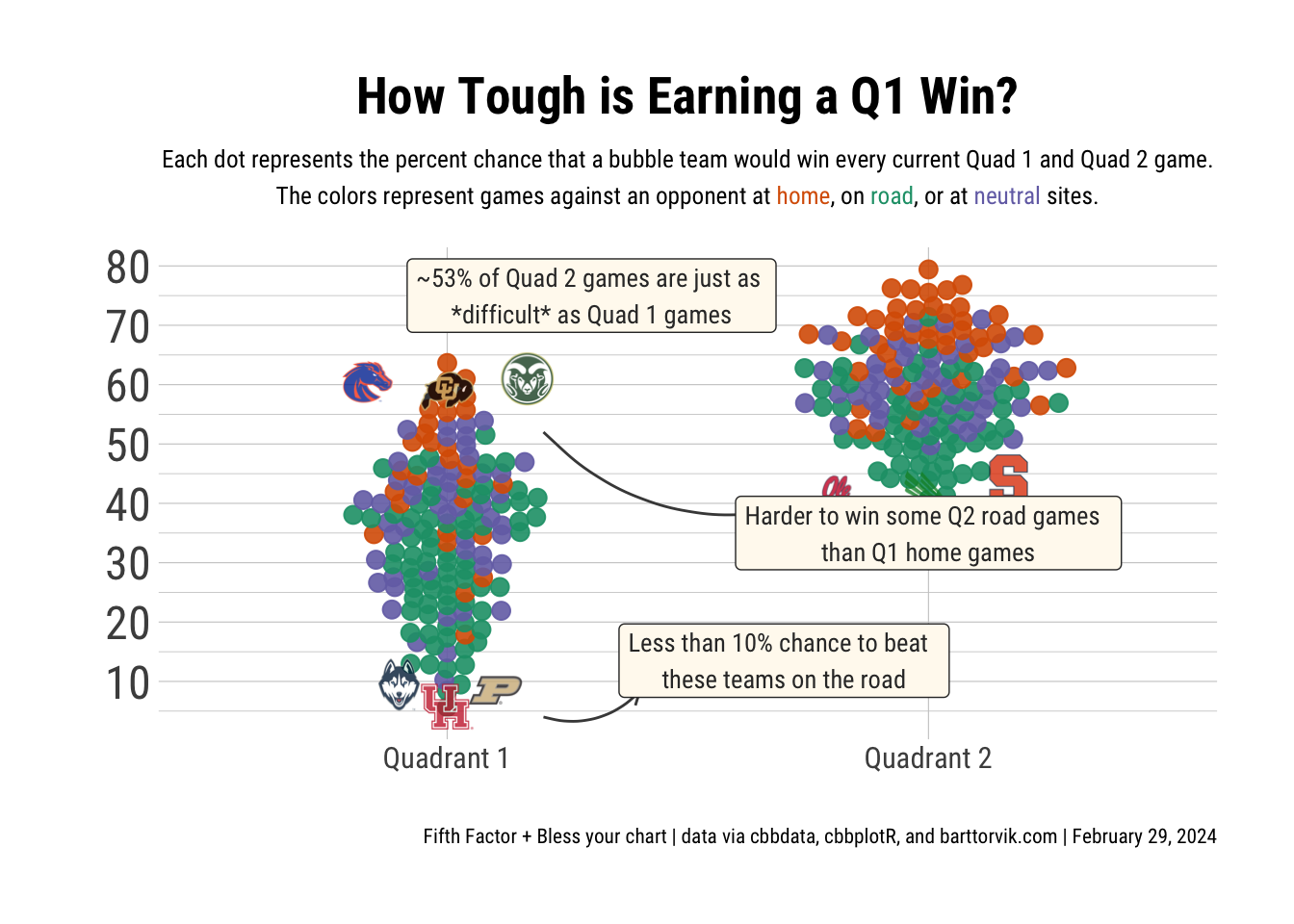
    title = "How Tough is Earning a Q1 Win?",
    subtitle = "Each dot represents the percent chance that a bubble team would win every current Quad 1 and Quad 2 game.  \nThe colors represent games against an opponent at <span style='color:#D95F02;'>home</span>, on <span style='color:#1B9E77; font-weight:bold'>road</span>, or at <span style='color:#7570B3'>neutral</span> sites.",
    x = "",
    y = "",
    caption = "Fifth Factor + Bless your chart | data via cbbdata, cbbplotR, and barttorvik.com | February 29, 2024"
  ) +
  ggplot2::scale_y_continuous(breaks = seq(0, 100, 10)) +
  ggplot2::labs(shape = "Quadrant") +
  ggplot2::scale_color_brewer(palette = "Dark2") +
  hrbrthemes::theme_ipsum_rc() +
  ggplot2::theme(
    plot.title = ggplot2::element_text(
      hjust = 0.5,
      size = 20,
      family = "Roboto Condensed"
    ),
    plot.subtitle = ggtext::element_markdown(
      hjust = 0.5,
      size = 9.5,
      lineheight = 1.5,
      family = "Roboto Condensed"
    ),
    legend.position = "none",
    axis.text.y = ggplot2::element_text(size = 18, family = "Roboto Condensed"),
    plot.caption = ggplot2::element_text(face = "plain", size = 8, "Roboto Condensed")
  ) +
  cbbplotR::geom_cbb_teams(
    data = func_data |>
      dplyr::arrange(bub_win_prob) |>
      dplyr::slice(1:3),
    ggplot2::aes(
      x = quad,
      y = 100 * bub_win_prob,
      team = opp
    ),
    width = .055,
    alpha = 0.8,
    position = ggplot2::position_dodge(width = 0.3)
  ) +
  cbbplotR::geom_cbb_teams(
    data = func_data |>
      dplyr::filter(quad == "Quadrant 1" & location == "H") |>
      dplyr::arrange(-bub_win_prob) |>
      dplyr::slice(2:4),
    ggplot2::aes(
      x = quad,
      y = 100 * bub_win_prob,
      team = opp
    ),
    width = .055,
    alpha = 0.8,
    position = ggplot2::position_dodge(width = 0.5)
  ) +
  cbbplotR::geom_cbb_teams(
    data = func_data |>
      dplyr::filter(quad == "Quadrant 2" & location == "A") |>
      dplyr::arrange(bub_win_prob) |>
      dplyr::slice(1:3),
    ggplot2::aes(
      x = quad,
      y = 100 * bub_win_prob,
      team = opp
    ),
    width = .055,
    alpha = 0.8,
    position = ggplot2::position_dodge(width = 0.5)
  ) +
  ggplot2::annotate(
    "label",
    x = 1.3,
    y = 75,
    label = "~53% of Quad 2 games are just as \n*difficult* as Quad 1 games",
    size = 3.5,
    color = "#333333",
    family = "Roboto Condensed",
    fill = "floral white"
  ) +
  ggplot2::annotate(
    geom = "curve",
    color = "#474747",
    x = 1.2,
    y = 4,
    xend = 1.4,
    yend = 8.3,
    curvature = .3,
    arrow = ggplot2::arrow(length = grid::unit(2, "mm"))
  ) +
  ggplot2::annotate(
    "label",
    x = 1.7,
    y = 13.5,
    label = "Less than 10% chance to beat  \nthese teams on the road",
    size = 3.5,
    color = "#333333",
    family = "Roboto Condensed",
    fill = "floral white"
  ) +
  ggplot2::annotate(
    geom = "curve",
    color = "#474747",
    x = 1.2,
    y = 52,
    xend = 1.75,
    yend = 40,
    curvature = .3,
    arrow = ggplot2::arrow(length = grid::unit(2, "mm"))
  ) +
  ggplot2::annotate(
    "label",
    x = 2,
    y = 35,
    label = "Harder to win some Q2 road games  \nthan Q1 home games",
    size = 3.5,
    color = "#333333",
    family = "Roboto Condensed",
    fill = "floral white"
  ) -> quad_plot

ggplot2::ggsave(
  "quad_plot.png",
  quad_plot,
  w = 7.5,
  h = 9.5,
  dpi = 300,
  type = 'cairo'
)

quad_plot

UK Bama plot