079: Possession plots

Data

library(cbbplotR)

# add in acc possessions
acc_poss <- readr::read_csv("https://gist.githubusercontent.com/gallochris/38a0da6c27978383e6b9502f14d2b1ca/raw/23438ef94cec0d5e405cc75c06fb56dbb0c8f0f9/unc_acc_poss.csv")

# fetch kentucky/bama game somehow 
schedule <- bigballR::get_team_schedule(season = "2023-24", team.name = "Kentucky")

================================================================================

ukbama_pbp <-bigballR::get_play_by_play(schedule$Game_ID[27])

ukbama_poss <- bigballR::get_possessions(play_by_play_data = ukbama_pbp)

UVA-UNC plot

uva_poss <- acc_poss |>
  dplyr::filter(ID == 5629143) |>
  dplyr::mutate(scoring = dplyr::if_else(PTS > 0, TRUE, FALSE))

row_index <- which(uva_poss$Half_Status == 2)[1]

first_poss_num <- uva_poss$Poss_Num[row_index] / 2

uva_unc_plot <- uva_poss |>
  ggplot2::ggplot(ggplot2::aes(x = Poss_Num / 2, y = Poss_Team, fill = scoring)) +
  ggplot2::geom_tile(width = 0.75, height = 0.25) +
  ggplot2::scale_fill_manual(values = c("lightpink", "lightgreen")) +
  ggplot2::scale_x_continuous(breaks = seq(0, 60, 5), limits = c(0, 65)) +
  ggplot2::geom_vline(xintercept = first_poss_num,
                      linetype = "dashed",
                      color = "#333333") +
  ggplot2::annotate(
    "rect",
    fill = "yellow",
    alpha = 0.35,
    xmin = 11.5 / 2,
    xmax = 24.5 / 2,
    ymin = -Inf,
    ymax = Inf
  ) +
  ggplot2::theme_classic() +
  ggplot2::theme(legend.position = "none",
                 axis.text.y = cbbplotR::element_cbb_teams(size = 0.9)) +
  ggplot2::labs(
    x = "Possessions",
    y = "",
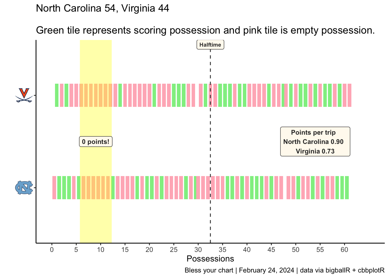
    title = "North Carolina 54, Virginia 44
                  \nGreen tile represents scoring possession and pink tile is empty possession.",
    caption = "Bless your chart | February 24, 2024 | data via bigballR + cbbplotR"
  ) +
  ggplot2::annotate(
    "label",
    x = 108 / 2,
    y = 1.5,
    label = "Points per trip  \nNorth Carolina 0.90  \nVirginia 0.73",
    size = 3,
    color = "#333333",
    fill = "floralwhite",
    fontface = "bold"
  ) +
  ggplot2::annotate(
    "label",
    x = 18 / 2,
    y = 1.5,
    label = "0 points!",
    size = 3,
    color = "#333333",
    fill = "floralwhite",
    fontface = "bold"
  ) +
  ggplot2::annotate(
    "label",
    x = first_poss_num,
    y = 2.55,
    label = "Halftime",
    size = 2.5,
    color = "#333333",
    fill = "floralwhite",
    fontface = "bold"
  ) 

uva_unc_plot

ggplot2::ggsave(
  "uva-plot.png",
  uva_unc_plot,
  w = 10,
  h = 6,
  dpi = 300,
  type = 'cairo'
)

UK Bama plot

# ukbama plot 
ukbama <- ukbama_poss |>
  dplyr::mutate(scoring = dplyr::if_else(PTS > 0, TRUE, FALSE))

# find half time
ukbama_row_index <- which(ukbama$Half_Status == 2)[1]

ukbama_poss_num <- ukbama$Poss_Num[ukbama_row_index] / 2

ukbama_plot <- ukbama |>
  ggplot2::ggplot(ggplot2::aes(x = Poss_Num / 2, y = Poss_Team, fill = scoring)) +
  ggplot2::geom_tile(width = 0.75, height = 0.25) +
  ggplot2::scale_fill_manual(values = c("lightpink", "lightgreen")) +
  ggplot2::scale_x_continuous(breaks = seq(0, 85, 5), limits = c(0, 85)) +
  ggplot2::geom_vline(xintercept = ukbama_poss_num,
                      linetype = "dashed",
                      color = "#333333") +
  ggplot2::annotate(
    "rect",
    fill = "yellow",
    alpha = 0.35,
    xmin = 92.5 / 2,
    xmax = 105.5 / 2 - .7,
    ymin = -Inf,
    ymax = Inf
  ) +
  ggplot2::theme_classic() +
  ggplot2::theme(legend.position = "none",
                 axis.text.y = cbbplotR::element_cbb_teams(size = 0.9)) +
  ggplot2::labs(
    x = "Possessions",
    y = "",
    title = "Kentucky 117, Alabama 95
                  \nGreen tile represents scoring possession and pink tile is empty possession.",
    caption = "Bless your chart | February 24, 2024 | data via bigballR + cbbplotR"
  ) +
  ggplot2::annotate(
    "label",
    x = 152 / 2,
    y = 1.5,
    label = "Points per trip  \nKentucky 1.46  \nAlabama 1.19",
    size = 3,
    color = "#333333",
    fill = "floralwhite",
    fontface = "bold"
  ) +
  ggplot2::annotate(
    "label",
    x = 99.5 / 2,
    y = 1.5,
    label = "12-0  \nKentucky  \nrun",
    size = 3,
    color = "#333333",
    fill = "floralwhite",
    fontface = "bold"
  ) +
  ggplot2::annotate(
    "label",
    x = ukbama_poss_num,
    y = 2.55,
    label = "Halftime",
    size = 2.5,
    color = "#333333",
    fill = "floralwhite",
    fontface = "bold"
  ) 

ukbama_plot 

ggplot2::ggsave(
  "ukbama-plot.png",
  ukbama_plot,
  w = 10,
  h = 6,
  dpi = 300,
  type = 'cairo'
)