077: ACC race and differentials

Data

library(cbbplotR)
# add all acc teams and leaders
acc_teams <- c("North Carolina", "Duke", "Virginia", "Clemson", "Wake Forest",
               "Virginia Tech", "Georgia Tech", "Florida St.", "Syracuse", 
               "North Carolina St.", "Boston College", "Louisville", 
               "Miami FL", "Notre Dame", "Pittsburgh")

leaders <- c("North Carolina", "Duke", "Virginia")

# fetch current ACC results 
acc_results <- cbbdata::cbd_torvik_game_stats(year = 2024, type = "conf") |> 
  dplyr::filter(conf == "ACC") |> 
  dplyr::select(date, team, opp, location, result, pts_scored, pts_allowed)

# fetch future acc schedule 
playedGames <-
  cbbdata::cbd_torvik_game_stats(year = "2024")$game_id |> 
  unique()

home_future <-
  cbbdata::cbd_torvik_season_schedule(year = "2024") |>
  dplyr::filter(!game_id %in% playedGames & type != "nond1") |>
  dplyr::mutate(team = home, opp = away) |> 
  dplyr::mutate(location = "H") |> 
  dplyr::filter(type == "conf") |> 
  dplyr::filter(team %in% acc_teams) |> 
  dplyr::select(date, team, opp, location) 

away_future <-
  cbbdata::cbd_torvik_season_schedule(year = "2024") |>
  dplyr::filter(!game_id %in% playedGames & type != "nond1") |>
  dplyr::mutate(team = away, opp = home) |> 
  dplyr::mutate(location = "A") |> 
  dplyr::filter(type == "conf") |> 
  dplyr::filter(team %in% acc_teams) |> 
  dplyr::select(date, team, opp, location) 


# combine data with differentials and game number/location
acc_sched <-
  rbind.data.frame(home_future, away_future) |>
  dplyr::bind_rows(acc_results) |> 
  dplyr::group_by(team) |> 
  dplyr::arrange(date) |> 
    dplyr::mutate(dplyr::across(everything(), ~ replace(.x, is.na(.x), ""))) |> 
  dplyr::mutate(game_num = dplyr::row_number(), 
                score = dplyr::if_else(result == "W" | result == "L", 
                  paste0(pts_scored, "-", pts_allowed),
                  "")) |> 
  dplyr::ungroup() |> 
  dplyr::select(game_num, team, opp, result, location, score) |> 
  dplyr::mutate(location = dplyr::if_else(location == "A", "Away", "Home"),
                text_label = paste0(result, "\n", score, "\n", location),
                game_num = as.numeric(game_num))

# add labels 
acc_sched |> 
  dplyr::filter(!is.na(result)) |> 
  dplyr::group_by(team) |> 
  dplyr::summarise(
    wins = sum(result == "W"),
    loss = sum(result == "L")
  ) |> 
  dplyr::filter(team %in% leaders) |> 
  dplyr::mutate(record = paste0(wins, "-", loss),
                game_num = -.5,
                result = "") |> 
  dplyr::select(team, game_num, record, result) -> rec_labels


# Differential table 
acc_diffs <- cbbdata::cbd_torvik_game_stats(year = 2024, type = "conf") |> 
  dplyr::filter(conf == "ACC") |> 
  dplyr::select(date, team, opp, location, result, pts_scored, pts_allowed) |> 
  dplyr::group_by(team) |> 
  dplyr::arrange(date) |> 
  dplyr::mutate(game_num = dplyr::row_number(), 
                diff = cumsum(pts_scored - pts_allowed)) |> 
  dplyr::ungroup()
  
acc_full_diffs <- acc_diffs |>   
  dplyr::add_row(data.frame(
    team = unique(acc_diffs$team),
    date = as.Date("2024-01-01"),  # Placeholder date, adjust as needed
    opp = NA,
    location = NA,
    result = NA,
    pts_scored = NA,
    pts_allowed = NA,
    game_num = 0,
    diff = 0
  ))

acc_last <- acc_diffs |> 
      dplyr::group_by(team) |> 
      dplyr::filter(game_num == max(game_num))

Theme

theme_me <- function() {
  # Create a base theme with minimal style
  base_theme <- ggplot2::theme_minimal(base_size = 10, base_family = "RobotoCondensed-Regular")
  
  # Customize the base theme with additional modifications
  custom_theme <- base_theme +
    ggplot2::theme(
      legend.position = "none", 
                 plot.title = ggtext::element_markdown(size = 18, face ='bold', family = 'mono'),
                 plot.subtitle = ggtext::element_markdown(size = 10, family = "mono", face = "bold"),
                 plot.caption = ggtext::element_markdown(size = 7, family = 'mono'),
      plot.background = ggplot2::element_rect(fill = "floralwhite", color = "floralwhite")
    )
  return(custom_theme)
} 

Geom Tile

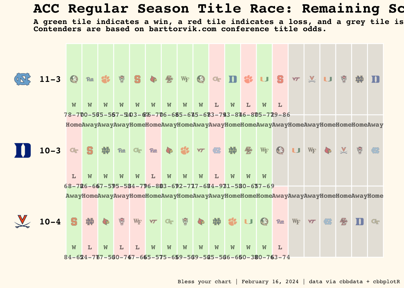
race_plot <- acc_sched |>
  dplyr::filter(team %in% c("North Carolina", "Duke", "Virginia")) |>
  dplyr::mutate(team = forcats::fct_relevel(
    team,
    c("Virginia", "Duke", "North Carolina")
  )) |>
  ggplot2::ggplot(ggplot2::aes(
    x = team,
    y = game_num,
    fill = factor(result)
  )) +
  ggplot2::scale_fill_manual(values = c(
    W = ggplot2::alpha("lightgreen", 0.3),
    L = ggplot2::alpha("lightpink", 0.3),
    ggplot2::alpha("#acacac", 0.3)
  )) +
  ggplot2::geom_tile(color = "white",
                     linewidth = .5,
                     height = 1) +
  ggplot2::geom_text(
    ggplot2::aes(label = text_label),
    fontface = "bold",
    family = "mono",
    alpha = 0.6,
    size = 3,
    vjust = 2
  ) +
  cbbplotR::geom_cbb_teams(ggplot2::aes(team = opp, y = game_num),
                           width = 0.025,
                           alpha = .5) +
  theme_me() +
  ggplot2::theme(
    legend.position = "none",
    axis.text.y = cbbplotR::element_cbb_teams(size = 0.8),
    axis.text.x = ggplot2::element_blank(),
    panel.grid = ggplot2::element_blank()
  ) +
    ggplot2::geom_text(
    data = rec_labels,
    ggplot2::aes(x = team, y = game_num, label = record),
    fontface = "bold",
    family = "mono",
    size = 4,
  ) +
  ggplot2::labs(
    x = "",
    y = "",
    title = "ACC Regular Season Title Race: Remaining Schedule of Top 3 Contenders",
    subtitle = "A green tile indicates a win, a red tile indicates a loss, and a grey tile is a scheduled game.  \nContenders are based on barttorvik.com conference title odds.",
    caption = "Bless your chart | February 16, 2024 | data via cbbdata + cbbplotR"
  ) +
  ggplot2::coord_flip() 


ggplot2::ggsave(
  "race-plot.png",
  race_plot,
  w = 12,
  h = 8,
  dpi = 300,
  type = 'cairo'
)

race_plot

Differential line plot

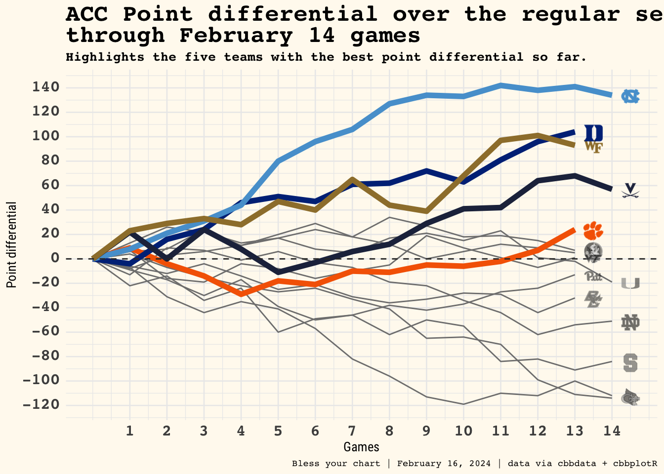
signal_teams <- c("Duke", "North Carolina", "Wake Forest", "Virginia", "Clemson")

acc_full_diffs |> 
  ggplot2::ggplot(ggplot2::aes(x = game_num, y = diff, color = team)) +
  ggplot2::geom_line(linewidth = 0.5) +
  ggplot2::geom_line(data = acc_full_diffs |> dplyr::filter(team %in% signal_teams), linewidth = 2) +
  ggplot2::scale_color_manual(values = c("North Carolina" = "#56a0d3",
                                         "Duke" = "#003087",
                                         "Wake Forest" = "#9E7E38",
                                         "Virginia" = "#232D4B",
                                         "Clemson" = "#F56600",
                                         Other = "#eeeeee")) +
  ggplot2::geom_hline(yintercept = 0, linetype = "dashed", color = "#333333") +
  ggplot2::scale_x_continuous(breaks = seq(1, 14, 1)) +
  ggplot2::scale_y_continuous(breaks = seq(-140, 140, 20)) +
  cbbplotR::geom_cbb_teams(
    data = acc_last,
    highlight_teams = signal_teams,
    ggplot2::aes(
    x = game_num + .5,
    y = diff - .99,
    team = team),
    width = .035,
    alpha = 0.6,
    highlight_method = "both"
  ) +
  theme_me() + 
  ggplot2::theme(legend.position = "none", 
                axis.text.x = ggtext::element_markdown(size = 12, family = 'mono', face ='bold'),  
                 axis.text.y = ggtext::element_markdown(size = 12, family = 'mono', face ='bold'),) +
  ggplot2::labs(title = "ACC Point differential over the regular season  \nthrough February 14 games",
                subtitle = "Highlights the five teams with the best point differential so far.",
                x = "Games",
                y = "Point differential",
                caption = "Bless your chart | February 16, 2024 | data via cbbdata + cbbplotR") -> diff_chart 

ggplot2::ggsave(
  "diff-plot.png",
  diff_chart,
  w = 10,
  h = 8,
  dpi = 300,
  type = 'cairo'
)

diff_chart