072: Free Throws

Data

# snag data from cbbdata
bacot <- cbbdata::cbd_torvik_player_game(player = "Armando Bacot") |> 
         dplyr::mutate(exp = dplyr::if_else(
             date > "2023-11-05", "Grad", exp)) 


# compute cumulative rates
ft_rates <- bacot |> 
        dplyr::mutate(fga = two_a + three_a, 
                      ft_rate = 100 * (fta/fga),
                      ft_pct = 100 * (ftm / fta),
                      row_num = dplyr::row_number(),
                      cume_pct = cumsum(ft_pct)) |> 
        dplyr::mutate(yr = dplyr::case_match(exp,
                    "Grad" ~ 2024, 
                    "Sr" ~ 2023, 
                    "Jr" ~ 2022,
                    "So" ~ 2021, 
                    "Fr" ~ 2020)) |> 
       dplyr::select(row_num, date, player, yr, 
                     opp, ft_rate, fga, ftm, fta, ft_pct, cume_pct)
# find cumulative makes
ft_rates |> 
  dplyr::group_by(yr) |> 
  dplyr::mutate(makes = cumsum(ftm),
                attempts = cumsum(fta),
                pct = makes/attempts,
                game_no = dplyr::row_number()) |>
  dplyr::select(game_no, yr, date, opp, makes, attempts, pct) -> cume_makes

# add annotations
pct_text <- data.frame(
  yr=c(2020,2021,2022,2023),
  game_no=c(10,10,10,10),
  makes = c(150,150,150,150),
  label=c("64.5%",
          "66.4%", 
          "67.0%", 
          "66.5%")
)

special_text <- data.frame(
  yr=c(2024),
  game_no=c(10),
  makes = c(150),
  label=c("79.8%")
)

ftm_text <-data.frame(
  yr=c(2020,2021,2022,2023,2024),
  game_no=c(10,10,10,10,10),
  makes = c(140,140,140,140,140),
  label=c("80-124",
          "84-127", 
          "146-218", 
          "139-209", 
          "79-99")
)

Small multiples

theme_me <- function() {
  base_theme <- ggplot2::theme_minimal(base_size = 10, base_family = "RobotoCondensed-Regular")
  
  custom_theme <- base_theme +
    ggplot2::theme(
      plot.title = ggplot2::element_text(
        hjust = 0.5,
        size = 24,
        face = "bold"
      ),
      plot.subtitle = ggplot2::element_text(
        hjust = 0.5,
        size = 10,
      ),
      plot.caption = ggplot2::element_text(
        hjust = 0.5,
        size = 6,
        lineheight = 0.35,
        margin = ggplot2::margin(t = 0.5)
      ),
      plot.background = ggplot2::element_rect(fill = "floralwhite", color = "floralwhite")
    )
  
  return(custom_theme)
} 

cume_makes |>
  ggplot2::ggplot(ggplot2::aes(x = game_no)) +
  ggplot2::geom_line(ggplot2::aes(y = makes), color = "#56a0d3") +
  ggplot2::geom_line(ggplot2::aes(y = attempts), color = "#333333") +
  ggplot2::facet_wrap(
    ~ yr,
    nrow = 2,
    strip.position = "top",
    labeller = ggplot2::labeller(
      yr = c(
        "2024" = "2023-24",
        "2023" = "2022-23",
        "2022" = "2021-22",
        "2021" = "2020-21",
        "2020" = "2019-20"
      )
    )
  ) +
  ggplot2::geom_text(
    data = pct_text,
    x = 10,
    y = 150,
    label = pct_text$label,
    color = "#333333",
    size = 4.5,
    fontface = 'bold',
    family = 'mono'
  ) +
  ggplot2::geom_text(
    data = special_text,
    x = 10,
    y = 150,
    label = special_text$label,
    color = "#56a0d3",
    size = 5.5,
    fontface = 'bold',
    family = 'mono'
  ) +
  ggplot2::geom_text(
    data = ftm_text,
    x = 9.7,
    y = 130,
    label = ftm_text$label,
    color = "#333333",
    size = 3,
    fontface = 'bold',
    family = 'mono'
  ) +
  ggplot2::labs(
    x = "Games",
    y = "",
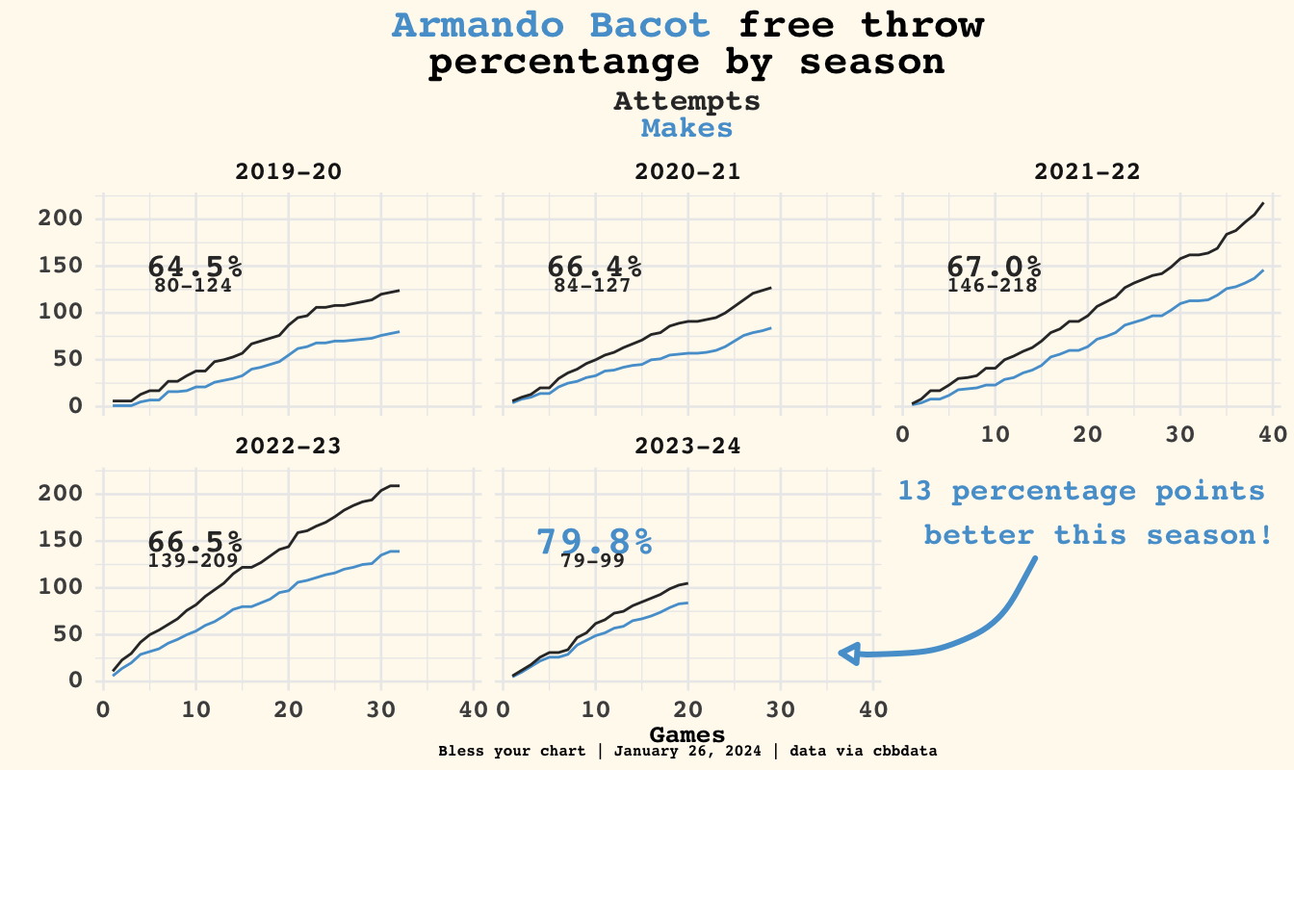
    title = "<span style='color:#56a0d3;'>Armando Bacot</span> free throw  \npercentange by season",
    subtitle = "<span style='color:#333333;'>Attempts</span>  \n<span style='color:#56a0d3;'>Makes</span>",
    caption = "Bless your chart | January 26, 2024 | data via cbbdata"
  ) +
  theme_me() +
  ggplot2::theme(
    plot.title = ggtext::element_markdown(
      size = 16,
      face = 'bold',
      family = 'mono'
    ),
    plot.subtitle = ggtext::element_markdown(
      size = 12,
      face = 'bold',
      family = 'mono'
    ),
    plot.caption = ggtext::element_markdown(
      size = 6,
      face = 'bold',
      family = 'mono'
    ),
    axis.text.x = ggtext::element_markdown(
      size = 10,
      face = 'bold',
      family = 'mono'
    ),
    axis.title.x = ggtext::element_markdown(
      size = 10,
      face = 'bold',
      family = 'mono'
    ),
    axis.text.y = ggtext::element_markdown(
      size = 10,
      face = 'bold',
      family = 'mono'
    ),
    strip.text.x = ggtext::element_markdown(
      size = 10,
      face = 'bold',
      family = 'mono'
    )
  ) -> mando_plot

# Add more annotations 
mondo_grob <- grid::textGrob("13 percentage points  \nbetter this season!",
                             x = 0.85, y = 4.35,
                             gp = grid::gpar(fontsize = 12, 
                                             col = "#56a0d3",
                                             fontface = 'bold',
                                             fontfamily = 'mono'))

curve_path <- grid::curveGrob(x1 = 0.80, y1 = 4.75, x2 = 0.67, y2 = 3.5,
                              curvature = -0.3, 
                              gp = grid::gpar(col = "#56a0d3", lwd = 3, fontfamily = 'mono'))

arrow_head <- grid::segmentsGrob(
  x1 = 0.65, y0 = 3.5,  
  x0 = 0.67, y1 = 3.52, 
  arrow = grid::arrow(length = ggplot2::unit(0.1, "inches"), type = "closed"),
  gp = grid::gpar(col = "#56a0d3", lwd = 3, fontfamily = 'mono')
)

curved_arrow <- grid::grobTree(curve_path, arrow_head)

cowplot::plot_grid(
  mando_plot,
  mondo_grob,
  curved_arrow,
  nrow = 3,
  rel_heights = c(1,0.1, 0.1) 
) -> plot_final

ggplot2::ggsave(
  "plot_final.png",
  plot_final,
  w = 8,
  h = 8,
  dpi = 600,
  type = 'cairo'
)

plot_final