061: Q1 last season

Load data

net_last <- readr::read_csv("net_2023_szn.csv") 

net_last |> 
  dplyr::mutate(real_date = lubridate::mdy(date))  |> 
  dplyr::group_by(conf, real_date) |> 
  dplyr::reframe(quad_ones = sum(q1_win + q1_loss),
                 quad_twos = sum(q2_win + q2_loss), 
                 quad_threes = sum(q3_win + q3_loss),
                 quad_fours = sum(q4_win + q3_loss)) -> conf_q1

Theme

theme_me <- function() {
  # Create a base theme with minimal style
  base_theme <- ggplot2::theme_minimal(base_size = 10, base_family = "RobotoCondensed-Regular")
  
  # Customize the base theme with additional modifications
  custom_theme <- base_theme +
    ggplot2::theme(
      plot.title = ggplot2::element_text(
        hjust = 0.5,
        size = 24,
        face = "bold"
      ),
      plot.subtitle = ggplot2::element_text(
        hjust = 0.5,
        size = 10,
        lineheight = 0.25,
        vjust = -0.5
      ),
      plot.caption = ggplot2::element_text(
        hjust = 0.5,
        size = 6,
        lineheight = 0.35,
        margin = ggplot2::margin(t = 0.5)
      ),
      plot.background = ggplot2::element_rect(fill = "floralwhite", color = "floralwhite")
    )
  
  return(custom_theme)
} 

Line chart

conf_levels <- conf_q1 |>
  dplyr::filter(conf %in% c("ACC", "Big 12", "SEC", 
                            "Pac-12", "Big Ten", "Big East")) |> 
  dplyr::filter(real_date == "2023-03-12") |> 
  dplyr::arrange(desc(quad_ones)) |>
  dplyr::pull(conf)

conf_lables <- conf_q1 |>
  dplyr::filter(conf %in% c("ACC", "Big 12", "SEC", 
                            "Pac-12", "Big Ten", "Big East")) |> 
  dplyr::filter(real_date == "2023-03-12") |> 
  dplyr::arrange(desc(quad_ones)) |>
  dplyr::select(conf, quad_ones, real_date)


conf_q1 |> 
  dplyr::filter(conf %in% c("ACC", "Big 12", "SEC", 
                            "Pac-12", "Big Ten", "Big East")) |>
  dplyr::mutate(conf = factor(conf, levels = conf_levels)) |> 
  ggplot2::ggplot(ggplot2::aes(x = real_date, y = quad_ones, group = conf)) +
  ggplot2::geom_line(color = "#333333", linewidth = 1) +
  ggplot2::scale_y_continuous(breaks = seq(0, 200, 50)) +
  ggplot2::facet_wrap(~conf, nrow = 3)  +
  ggplot2::geom_text(
    data = conf_lables |> 
      dplyr::mutate(conf = factor(conf, levels = conf_levels)),
    y = 185,
    x = as.Date("2023-01-25"),
    label=conf_lables$quad_ones,
    color = "#333333",
    fontface = "bold",
    family = "mono"
  ) + 
  theme_me() +
  ggplot2::theme(legend.position = "none", 
                 plot.title = ggtext::element_markdown(face ='bold', family = 'mono'),
                 strip.text.x = ggtext::element_markdown(size = 12, 
                                                         face ='bold', family = 'mono'),
                 plot.caption = ggtext::element_markdown(size = 7, family = 'mono'),
                 axis.text.x = ggtext::element_markdown(size = 10, family = 'mono'),  
                 axis.text.y = ggtext::element_markdown(size = 10, family = 'mono')
  ) +
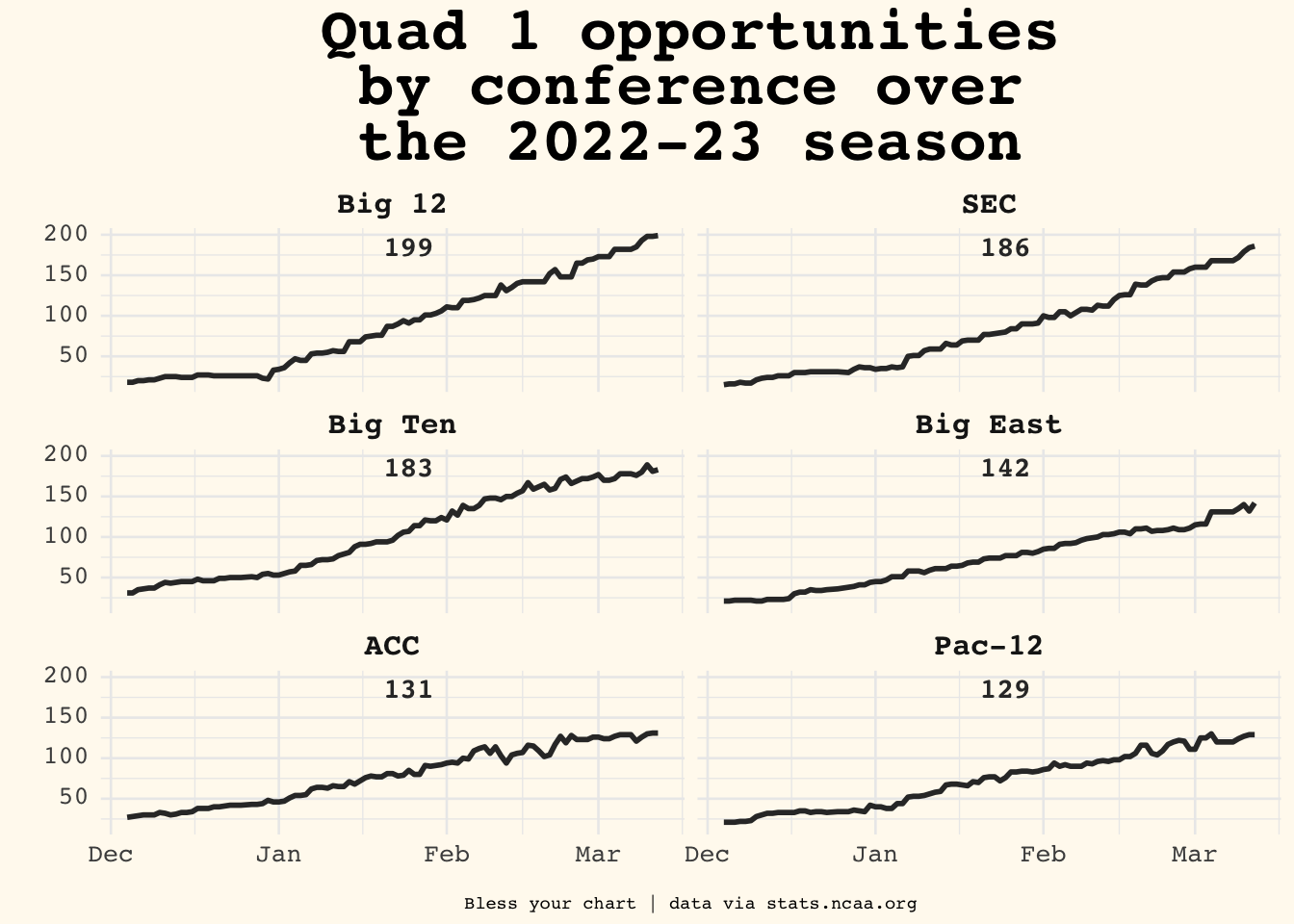
  ggplot2::labs(x = "",
                y = "",
                title = "Quad 1 opportunities  \nby conference over  \nthe 2022-23 season",
                caption = "Bless your chart | data via stats.ncaa.org"
  ) -> conf_plot 


ggplot2::ggsave(
  "conf_plot.png",
  conf_plot,
  w = 6.5,
  h = 8.5,
  dpi = 600,
  type = 'cairo'
)

conf_plot