056: Close Games

Load data

# fetch all regular season ACC games since 2005
combine_data <- function(years = year,
                         season_type = "regular",
                         conference = "ACC") {
  # Fetch the game data
  data <- lapply(years, function(year) {
    cfbfastR::cfbd_game_info(year = year,
                             season_type = season_type,
                             conference = conference) |>
      dplyr::filter(conference_game == TRUE) |>
      dplyr::select(season,
                    week,
                    home_team,
                    home_points,
                    away_team,
                    away_points)
  })
  
  # Bind the data together
  data <- dplyr::bind_rows(data)
  # Filter out any rows with missing values for home_points
  data <- data |> dplyr::filter(!is.na(home_points))
  # Return the data
  return(data)
}

# find records since 2005
last_10_seasons <- c(2005:2023)
acc_data <- combine_data(years = last_10_seasons)

# filter out conference champ games
# filter out non-conference conference games
# filter out Notre Dame in 2021
reg_acc_data <- acc_data |>
  dplyr::group_by(season) |>
  dplyr::mutate(max_week_number = max(week)) |>
  dplyr::mutate(max_week_number =
                  dplyr::if_else(season == 2023, 15, max_week_number)) |>
  dplyr::filter(week < max_week_number) |>
  dplyr::filter(season != 2021 |
                  (home_team != "Notre Dame" &
                     away_team != "Notre Dame")) |>
  dplyr::filter(!(season == 2021 &
                    home_team == "North Carolina" &
                    week == 10))


# home win pct
home_win_pct <-
  reg_acc_data |>
  dplyr::group_by(season) |>
  dplyr::summarize(home_win_avg = mean(home_points > away_points))

# only close games
close_games <-
  reg_acc_data |>
  dplyr::mutate(point_diff = home_points - away_points) |>
  dplyr::filter(point_diff >= -8 & point_diff <= 8) |>
  dplyr::group_by(season) |>
  dplyr::summarize(close_games = dplyr::n())

# total games
total_games <-
  reg_acc_data |>
  dplyr::group_by(season) |>
  dplyr::summarize(total_games = dplyr::n())

# close game percentage
close_game_pct <- close_games |>
  dplyr::left_join(total_games, by = "season") |>
  dplyr::mutate(close_game_pct = close_games / total_games)

# only avg point differential
avg_point_diff <-
  reg_acc_data |>
  dplyr::group_by(season) |>
  dplyr::summarize(avg_point_diff = mean(abs(home_points - away_points)))

# combine the data
full_results <- home_win_pct |>
  dplyr::left_join(close_game_pct, by = "season") |> 
  dplyr::left_join(avg_point_diff, by = "season")

reg_acc_data |> 
    dplyr::mutate(point_diff = abs(home_points - away_points), 
                  result = dplyr::if_else(home_points > away_points, "W", "L")) -> scores_only

Plot theme

theme_me <- function() {
  # Create a base theme with minimal style
  base_theme <- ggplot2::theme_minimal(base_size = 10, base_family = "RobotoCondensed-Regular")
  
  # Customize the base theme with additional modifications
  custom_theme <- base_theme +
    ggplot2::theme(
      plot.title = ggplot2::element_text(
        hjust = 0.5,
        size = 24,
        face = "bold"
      ),
      plot.subtitle = ggplot2::element_text(
        hjust = 0.5,
        size = 10,
        lineheight = 0.25,
        vjust = -0.5
      ),
      plot.caption = ggplot2::element_text(
        hjust = 1,
        size = 6,
        lineheight = 0.35,
        margin = ggplot2::margin(t = 20)
      ),
      plot.background = ggplot2::element_rect(fill = "floralwhite", color = "floralwhite")
    )
  
  return(custom_theme)
} 

GT Athletic Theme

gt_theme_athletic <- function(gt_object, ...) {
  
  # get id, if one is passed through to use with CSS
  table_id <- subset(gt_object[['_options']], parameter == 'table_id')$value[[1]]
  
  table <- gt_object |> 
    # set table font
    gt::opt_table_font(
      font = list(
        gt::google_font('Spline Sans Mono'),
        gt::default_fonts()
      ),
      weight = 500
    ) |> 
    # set the column label font and style
    gt::tab_style(
      locations = gt::cells_column_labels(
        columns = gt::everything()
      ),
      style = gt::cell_text(
        font = gt::google_font('Work Sans'),
        weight = 650,
        size = gt::px(14),
        transform = 'uppercase', # column labels to uppercase
        align = 'left'
      )
    ) |> 
    gt::tab_style(
      locations = gt::cells_title('title'),
      style = gt::cell_text(
        font = gt::google_font('Work Sans'),
        weight = 650
      )
    ) |> 
    gt::tab_style(
      locations = gt::cells_title('subtitle'),
      style = gt::cell_text(
        font = gt::google_font('Work Sans'),
        weight = 500
      )
    ) |>
    # set think black column sep.
    gt::tab_style(
      style = gt::cell_borders(sides = 'left', weight = gt::px(0.5), color = 'black'),
      locations = gt::cells_body(
        # everything but the first column
        columns = c(-names(gt_object[['_data']])[1])
      )
    ) |> 
    # set thin dotted row sep.
    gt::tab_style(
      style = gt::cell_borders(sides = "top", color = 'black', weight = gt::px(1.5), style = 'dotted'),
      locations = gt::cells_body(
        rows = gt::everything()
      )
    )|>
    # left align cell text
    gt::cols_align(
      align = 'left',
      columns = gt::everything()
    ) |> 
    gt::tab_options(
      table.font.size = 14,
      column_labels.border.bottom.width = 2,
      column_labels.border.bottom.color = 'black',
      column_labels.border.top.color = 'white',
      row_group.border.bottom.color = 'white',
      table.border.top.style = 'none',
      table.border.bottom.style = 'none',
      heading.border.bottom.style = 'none',
      heading.align = 'left',
      heading.title.font.size = gt::px(30),
      source_notes.border.lr.style = 'none',
      source_notes.font.size = 10
    )
  
  # add css if table id is passed through
  table <- if(!is.null(table_id)) {
    table |> 
      # remove the border from the bottom cell
      gt::opt_css(
        paste0("#", table_id, " tbody tr:last-child {border-bottom: 2px solid #ffffff00;}"),
        add = TRUE
      )
  }
  
  return(table)
  
}

GT Table

result_table <- full_results |> 
  dplyr::select(season, total_games, home_win_avg, avg_point_diff) |> 
  dplyr::arrange(-season) |> 
  gt::gt() |> 
  gt::cols_label(# rename columns
    season = "Season",
    home_win_avg = "Home Win %", 
    avg_point_diff = "Avg. MOV",
    total_games = "Games") |> 
 gt::fmt_number(columns = home_win_avg,
             decimals = 3,
             use_seps = FALSE) |> 
   gt::fmt_number(columns = avg_point_diff,
             decimals = 2,
             use_seps = FALSE) |> 
  gt_theme_athletic() |> 
    gtExtras::gt_hulk_col_numeric(home_win_avg:avg_point_diff, trim = TRUE) |> 
    gtExtras::gt_highlight_rows(
    rows = c(4),
    fill = "#ffffd8",
    bold_target_only = TRUE,
    target_col = c(season)
  ) |> 
  gt::tab_header(title = "ACC football: average margin of victory and home win percentage by season") |> 
  gt::tab_source_note(source_note = "Bless your chart | November 4 | data via cfbfastR")

gtExtras::gtsave_extra(result_table,
                       filename = "result_table.png",
                       vwidth = 450)

result_table

ACC football: average margin of victory and home win percentage by season
Season	Games	Home Win %	Avg. MOV
2023	38	0.605	14.26
2022	55	0.509	13.42
2021	56	0.571	14.18
2020	70	0.629	17.36
2019	56	0.571	16.93
2018	56	0.536	17.75
2017	56	0.554	13.82
2016	56	0.464	17.48
2015	56	0.536	11.98
2014	56	0.518	14.05
2013	56	0.500	18.16
2012	48	0.604	15.83
2011	48	0.583	13.08
2010	48	0.542	14.44
2009	48	0.562	13.27
2008	48	0.583	10.77
2007	48	0.583	12.98
2006	48	0.583	13.08
2005	48	0.562	15.02
Bless your chart | November 4 | data via cfbfastR

GG Beeswarm

pd_plot <- scores_only |> 
    ggplot2::ggplot(ggplot2::aes(x = season)) + 
    ggbeeswarm::geom_quasirandom(
        data = scores_only |> dplyr::filter(result == "L"),
        mapping = ggplot2::aes(y = point_diff, x = season),
        stroke = 0.8,
        color = "#e41a1c",
        size = 3,
        shape = 1
    ) +
    ggbeeswarm::geom_quasirandom(
        data = scores_only |> dplyr::filter(result == "W"),
        mapping = ggplot2::aes(y = point_diff, x = season),
        stroke = 0.8,
        fill = "#4daf4a",
        size = 3,
        shape = 21
    ) +
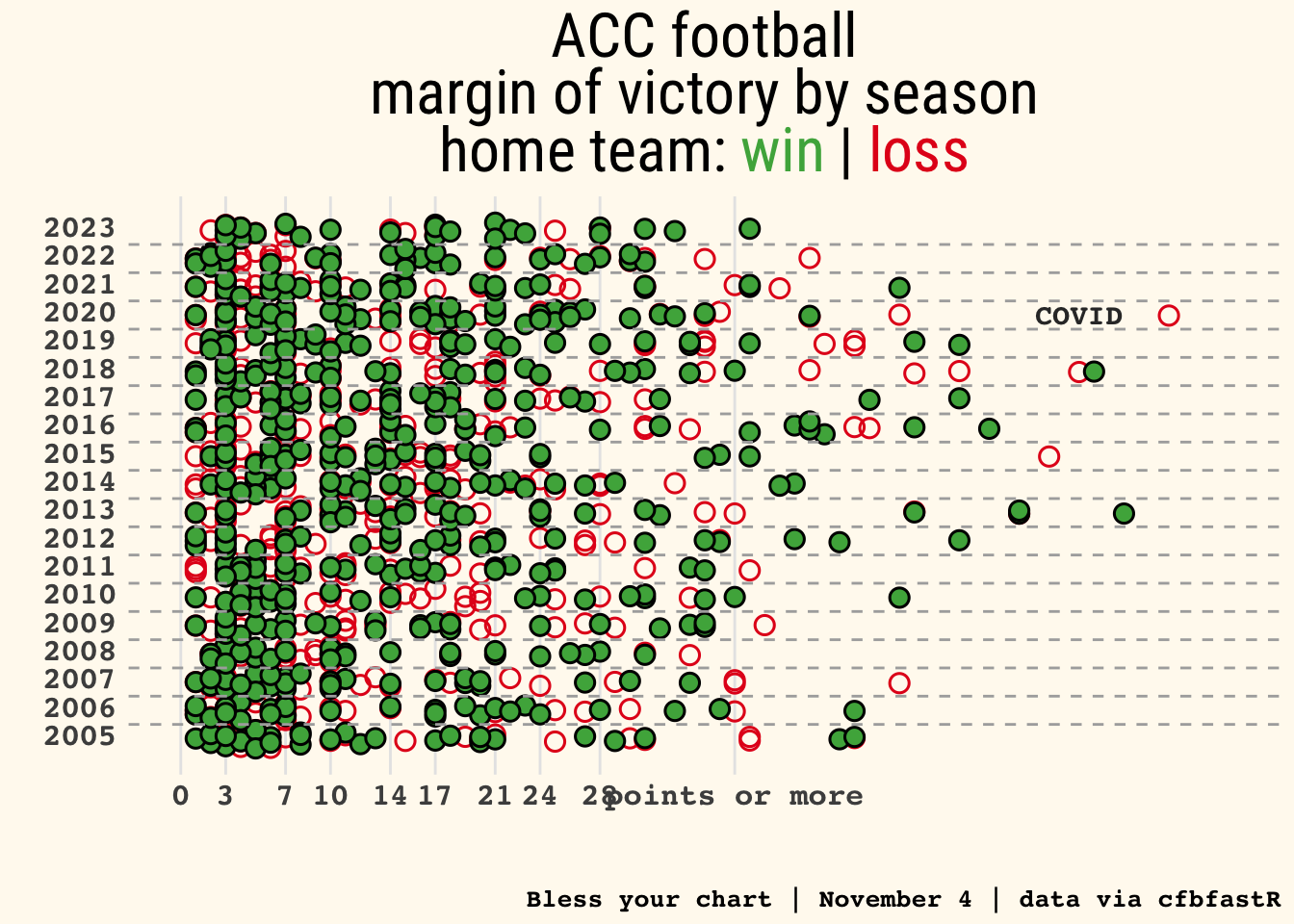
    ggplot2::scale_y_continuous(limits = c(0, 70), labels = c("0", "3", "7", "10", "14", "17", "21", "24", "28", "points or more"), breaks = c(0, 3, 7, 10, 14, 17, 21, 24, 28, 37)) +  
    ggplot2::scale_x_continuous(breaks = seq(2005, 2023, 1)) +
    ggplot2::coord_flip() +
    theme_me() +
    ggplot2::theme(legend.position = "none", 
                   plot.title = ggtext::element_markdown(),
                   plot.caption = ggtext::element_markdown(size = 10, face ='bold', family = 'mono'),
                   axis.text.x = ggtext::element_markdown(size = 12, face ='bold', family = 'mono'),  axis.text.y = ggtext::element_markdown(size = 12, face ='bold', family = 'mono'),
        panel.grid.major.x = ggplot2::element_line(color = "#E6E6E6", size = 0.5), 
                   panel.grid.minor.x = ggplot2::element_blank(),
                   panel.grid.major.y = ggplot2::element_blank(), 
                   panel.grid.minor.y = ggplot2::element_blank()) +
    ggplot2::geom_vline(xintercept = c(2005.5, 2006.5, 2007.5, 2008.5, 2009.5, 2010.5, 2011.5, 2012.5, 2013.5, 2014.5, 2015.5, 2016.5, 2017.5, 2018.5, 2019.5, 2020.5, 2021.5, 2022.5), 
                        color = "#acacac", linetype = "dashed") +
    ggplot2::labs(x = "",
                  y = "",
                  title = "ACC football  \nmargin of victory by season  \nhome team: <span style='color:#4daf4a;'>win</span> | <span style='color:#e41a1c;'>loss</span>",
                  caption = "Bless your chart | November 4 | data via cfbfastR"
                  ) +
   ggplot2::annotate(
        geom = "text",
        x = 2020,
        y = 60,
        color = "#333333",
        label = "COVID",
        size = 4,
        fontface = 'bold',
        family = 'mono'
    )


ggplot2::ggsave(
  "pd_plot.png",
  pd_plot,
  w = 8.5,
  h = 9.5,
  dpi = 600,
  type = 'cairo'
)

pd_plot