048: Third downs

Load data

# sc <- cfbfastR::cfbd_pbp_data(
#    2023,
#    season_type = "regular",
#    team = "North Carolina",
#    epa_wpa = TRUE,
#    week = 3
# ) |> 
#    dplyr::filter(offense_play == "North Carolina" & down == 3 & play_type != "Timeout")

# app <- cfbfastR::cfbd_pbp_data(
#    2023,
#    season_type = "regular",
#    team = "North Carolina",
#    epa_wpa = TRUE,
#    week = 3
# ) |> 
#    dplyr::filter(offense_play == "North Carolina" & down == 3 & play_type != "Timeout")

# minny <- cfbfastR::cfbd_pbp_data(
#    2023,
#    season_type = "regular",
#    team = "North Carolina",
#    epa_wpa = TRUE,
#    week = 3
# ) |> 
#    dplyr::filter(offense_play == "North Carolina" & down == 3 & play_type != "Timeout")

# nc_third_downs <- bind_rows(nc, app, minny) |> 
#     dplyr::filter(play_type != "Penalty")

# nc_third_downs |> 
#    dplyr::select(def_pos_team, distance, yards_gained) |> 
#    dplyr::mutate(conv = dplyr::if_else(yards_gained >= distance, "Yes", "No")) -> trd

# write.csv(trd, "unc-third-downs.csv)

unc_trd <- readr::read_csv("unc-third-downs.csv")

summary <- unc_trd |> 
    dplyr::group_by(def_pos_team, conv) |> 
    dplyr::summarise(count = dplyr::n()) |> 
    dplyr::mutate(conv = ifelse(conv == "Yes", "Converted", "Not Converted")) |> 
    tidyr::spread(key = conv, value = count, fill = 0) |> 
    dplyr::mutate(total_attempts = Converted + `Not Converted`,
           conversion_rate = Converted / total_attempts) |> 
    dplyr::rename(defense = def_pos_team, converted = Converted, attempts = total_attempts, rate = conversion_rate) |> 
    dplyr::select(-`Not Converted`)

Set the theme

theme_me <- function() {
  # Create a base theme with minimal style
  base_theme <- ggplot2::theme_minimal(base_size = 10, base_family = "RobotoCondensed-Regular")
  
  # Customize the base theme with additional modifications
  custom_theme <- base_theme +
    ggplot2::theme(
      plot.title = ggplot2::element_text(
        hjust = 0.5,
        size = 24,
        face = "bold"
      ),
      plot.subtitle = ggplot2::element_text(
        hjust = 0.5,
        size = 10,
        lineheight = 0.25,
        vjust = -0.5
      ),
      plot.caption = ggplot2::element_text(
        hjust = 1,
        size = 6,
        lineheight = 0.35,
        margin = ggplot2::margin(t = 20)
      ),
      plot.background = ggplot2::element_rect(fill = "floralwhite", color = "floralwhite")
    )
  
  return(custom_theme)
} 

UNC Third Downs

unc_trd |> 
    ggplot2::ggplot(ggplot2::aes(x = distance, y = yards_gained)) +
    ggplot2::geom_jitter(data = unc_trd |>  dplyr::filter(conv == "No"),
    mapping = ggplot2::aes(x = distance, y = yards_gained),
    stroke = 0.8,
    color = "#e41a1c",
    size = 3,
    shape = 1
  ) +
  ggplot2::geom_jitter(
    data = unc_trd |>  dplyr::filter(conv == "Yes"),
    mapping = ggplot2::aes(x = distance, y = yards_gained),
    stroke = 0.8,
    fill = "#4daf4a",
    size = 4,
    shape = 21
  ) +
  ggplot2::scale_x_continuous(breaks = seq(0, 25, 5), limits = c(0, 25)) +
  ggplot2::scale_y_continuous(breaks = seq(-10, 60, 10), limits = c(-10, 60)) +
  theme_me() +
  ggplot2::theme(legend.position = "none", plot.title = ggtext::element_markdown()) +
  ggplot2::labs(
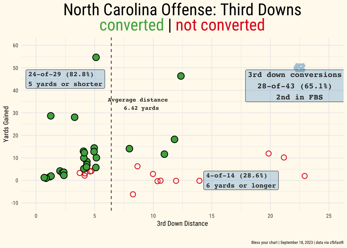
    x = "3rd Down Distance",
    y = "Yards Gained",
    title = "North Carolina Offense: Third Downs  \n<span style='color:#4daf4a;'>converted</span> | <span style='color:#e41a1c;'>not converted</span>",
    caption = "Bless your chart | September 18, 2023 | data via cfbfastR"
  ) +
  ggplot2::geom_vline(xintercept = 6.42,
             linetype = 'dashed',
             color = "#333333") -> plot_one 

full_plot <- plot_one + 
  ggplot2::annotate(
    cfbplotR::GeomCFBlogo,
    x = 22.5,
    y =50,
    team = "North Carolina",
    height = .075,
    alpha = 0.6
  ) +
  ggplot2::annotate(
    geom = "label",
    x = 22.5,
    y = 42,
    color = "#333333",
    fill = "#56a0d3",
    label = "3rd down conversions  \n28-of-43 (65.1%)  \n2nd in FBS",
    size = 4,
    fontface = 'bold',
    family = 'mono',
    alpha = 0.3
  ) +
  ggplot2::annotate(
    geom = "label",
    x = 2.5,
    y = 45,
    color = "#333333",
    fill = "#56a0d3",
    label = "24-of-29 (82.8%)  \n5 yards or shorter",
    size = 3.5,
    fontface = 'bold',
    family = 'mono',
    alpha = 0.3
  ) +
    ggplot2::annotate(
    geom = "label",
    x = 17.5,
    y = 0,
    color = "#333333",
    fill = "#56a0d3",
    label = "4-of-14 (28.6%)  \n6 yards or longer",
    size = 3.5,
    fontface = 'bold',
    family = 'mono',
    alpha = 0.3
  ) +
    ggplot2::annotate(
    geom = "text",
    x = 9,
    y = 34,
    color = "#333333",
    label = "Avgerage distance  \n6.42 yards",
    size = 3,
    fontface = 'bold',
    family = 'mono',
  ) 
  

ggplot2::ggsave(
  "trd.png",
  full_plot,
  w = 9,
  h = 8.5,
  dpi = 600,
  type = 'cairo'
)

full_plot