043: Scattershot

geom_tile
mapboxapi
Published

August 15, 2023

Fire up the data

Code
# WOMEN'S SOCCER DATA
file_path <- "~/byc/posts/byc_043/wsoc"

file_list <- list.files(file_path, pattern = "\\.xlsx$", full.names = TRUE)

# Create a function to read an Excel file and add a column with the file name
read_and_add_file_column <- function(file_path) {
  data <- readxl::read_excel(file_path, sheet = "Sheet1")
  data$file_name <- basename(file_path)  # Add a new column with the file name
  data
}

data_list <- purrr::map(file_list, read_and_add_file_column)

all_wsoc <- dplyr::bind_rows(data_list)

# teams to include 
ff_t <- c("UCLA", "Florida St.", "Southern California", "Penn St.", "Stanford", "Santa Clara", "Virginia", 
          "Duke", "West Virginia", "North Carolina", "BYU", "Virginia Tech",
          "Texas A&M", "Rutgers", "Georgetown", "South Carolina", "Washington State",
          "Alabama")

all_wsoc |> 
  dplyr::mutate(Team = gsub("\\([^)]*\\)", "", Team)) |> 
  dplyr::mutate(Team = trimws(Team)) |> 
  dplyr::filter(Team %in% ff_t) |> 
  dplyr::group_by(Team) |> 
  dplyr::mutate(W = cumsum(Won),
                L = cumsum(Lost), 
                Tie = cumsum(Tied),
                win_pct = (W + (.5 * Tie)) / (W + L + Tie)) |> 
  dplyr::filter(file_name == "22-23.xlsx") |> 
  dplyr::select(Team, W, L, Tie, win_pct) |> 
  dplyr::arrange(-win_pct) -> full_data

#. load titles
titles <- readr::read_csv("fdata.csv")

# join the data
wsoc_data <- dplyr::left_join(titles, full_data, by = "Team")

# load titles by season data set
haha <- readr::read_csv("haha.csv")

# NOTRE DAME DATA
get_notre_dame_stats <- function(start_year, end_year) {
  years <- start_year:end_year
  all_stats <- list()
  
  for (year in years) {
    stats <- cfbfastR::cfbd_game_team_stats(year, team = "Notre Dame")
    stats$year <- year  # Add a new column for the year
    all_stats[[as.character(year)]] <- stats
  }
  
  combined_stats <- dplyr::bind_rows(all_stats)
  
  return(combined_stats)
}

# Specify the range of years
start_year <- 2014
end_year <- 2022

# Get and combine game statistics for Notre Dame for the specified years
nd_stats <- get_notre_dame_stats(start_year, end_year)

# Sort the combined game statistics by year
nd_results <- nd_stats |> 
  dplyr::add_row(year = 2014, school = "Notre Dame", opponent = "LSU",
                 opponent_conference = "SEC", points = 31, points_allowed = 28) |> 
  dplyr::add_row(year = 2015, school = "Notre Dame", opponent = "Ohio State",
                 opponent_conference = "Big Ten", points = 28, points_allowed = 44) |> 
  dplyr::add_row(year = 2017, school = "Notre Dame", opponent = "LSU",
                 opponent_conference = "SEC", points = 21, points_allowed = 17) |> 
  dplyr::add_row(year = 2018, school = "Notre Dame", opponent = "Clemson",
                 opponent_conference = "ACC", points = 3, points_allowed = 30) |> 
  dplyr::add_row(year = 2019, school = "Notre Dame", opponent = "Iowa State",
                 opponent_conference = "Big 12", points = 33, points_allowed = 9) |> 
  dplyr::add_row(year = 2020, school = "Notre Dame", opponent = "Alabama",
                 opponent_conference = "SEC", points = 14, points_allowed = 31) |> 
  dplyr::add_row(year = 2021, school = "Notre Dame", opponent = "Oklahoma State",
                 opponent_conference = "Big 12", points = 35, points_allowed = 37) |> 
  dplyr::add_row(year = 2022, school = "Notre Dame", opponent = "South Carolina",
                 opponent_conference = "SEC", points = 45, points_allowed = 38) |> 
  dplyr::arrange(year) |> 
  dplyr::select(year, school, opponent, opponent_conference, home_away, points, points_allowed) |> 
  dplyr::mutate(diff = points -points_allowed) |> 
  dplyr::mutate(result = dplyr::if_else(diff > 0, "W", "L"))

Geom tile

Code
# make the tile chart
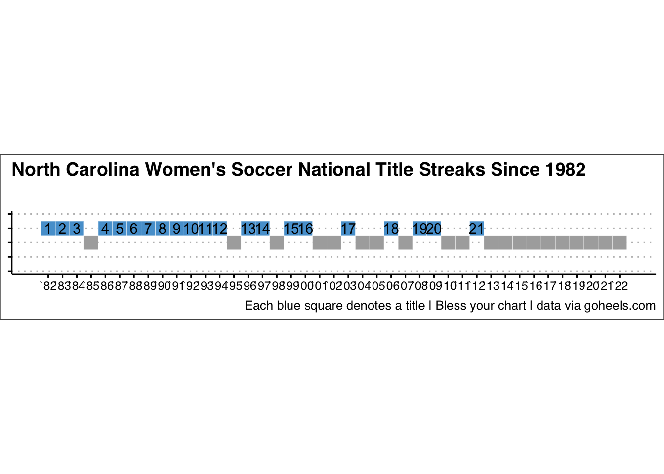
title_tile <- ggplot2::ggplot(haha, ggplot2::aes(x = year, y = title, fill = factor(title))) +
  ggplot2::geom_tile(color = "white") +
  ggplot2::scale_fill_manual(values = c("0" = "#acacac", "1" = "#56a0d3")) +
  ggplot2::geom_text(data = haha |> dplyr::filter(!is.na(count)), ggplot2::aes(label = count), color = "black") +
  ggplot2::scale_x_continuous(breaks = seq(1982, 2022, 1), labels = paste0("`", sprintf('%02d', 1982:2022 %% 100))) +
  ggplot2::scale_y_continuous(breaks = seq(-2, 2, 1), limits = c(-2, 2)) +
  ggplot2::coord_fixed(ratio = 1) + 
  ggthemes::theme_clean() +
  ggplot2::theme(axis.text.y = ggplot2::element_blank(), axis.title = ggplot2::element_blank(), 
        panel.grid = ggplot2::element_blank(),
        legend.position = "none") +
  ggplot2::labs(
    x = "",
    y = "",
    title = "North Carolina Women's Soccer National Title Streaks Since 1982",
    subtitle = "",
    caption = "Each blue square denotes a title | Bless your chart | data via goheels.com"
  ) 

title_tile

GT Table

Code
# gt theme from andrew https://gist.github.com/andreweatherman/3874a59a1f7b4af97e3699e4ece94579
gt_theme_athletic <- function(gt_object, ...) {
  
  gt_object |> 
    # set table font
    gt::opt_table_font(
      font = list(
        gt::google_font('Spline Sans Mono'),
        gt::default_fonts()
      ),
      weight = 500
    ) |> 
    # set the column label font and style
    gt::tab_style(
      locations = gt::cells_column_labels(
        columns = gt::everything()
      ),
      style = gt::cell_text(
        font = gt::google_font('Work Sans'),
        weight = 650,
        size = gt::px(14),
        transform = 'uppercase', # column labels to uppercase
        align = 'left'
      )
    ) |> 
    gt::tab_style(
      locations = gt::cells_title('title'),
      style = gt::cell_text(
        font = gt::google_font('Work Sans'),
        weight = 650
      )
    ) |> 
    gt::tab_style(
      locations = gt::cells_title('subtitle'),
      style = gt::cell_text(
        font = gt::google_font('Work Sans'),
        weight = 500
      )
    ) |>
    # set think black column sep.
    gt::tab_style(
      style = gt::cell_borders(sides = 'left', weight = gt::px(0.5), color = 'black'),
      locations = gt::cells_body(
        # everything but the first column
        columns = c(-names(gt_object[['_data']])[1])
      )
    ) |> 
    # set thin dotted row sep.
    gt::tab_style(
      style = gt::cell_borders(sides = "top", color = 'black', weight = gt::px(1.5), style = 'dotted'),
      locations = gt::cells_body(
        rows = gt::everything()
      )
    )|>
    # left align cell text
    gt::cols_align(
      align = 'left',
      columns = gt::everything()
    ) |> 
    gt::tab_options(
      table.font.size = 14,
      column_labels.border.bottom.width = 2,
      column_labels.border.bottom.color = 'black',
      column_labels.border.top.color = 'white',
      row_group.border.bottom.color = 'white',
      table.border.top.style = 'none',
      table.border.bottom.style = 'none',
      heading.border.bottom.style = 'none',
      heading.align = 'left',
      heading.title.font.size = gt::px(30),
      source_notes.border.lr.style = 'none',
      source_notes.font.size = 10
    ) |> 
    # remove the border from the bottom cell
    gt::opt_css(
      "tbody tr:last-child {
    border-bottom: 2px solid #ffffff00;
      }
    ",
      add = TRUE
    )
  
}

wsoc_data |>
  dplyr::mutate(Team = dplyr::case_match(Team, 
                       "Florida St." ~ "Florida State",
                       "Penn St." ~ "Penn State", 
                       "Southern California" ~ "USC",
                       .default = Team)) |> 
  dplyr::arrange(-win_pct) |>
  dplyr::mutate(logo = Team) |>
  dplyr::select(logo,
                Team,
                W,
                L,
                Tie,
                win_pct,
                titles,
                runnerup,
                semis) |>
  gt::gt() |>
  gt::cols_label(
    logo = "",
    Tie = "T",
    win_pct = "Win %",
    titles = "Titles",
    runnerup = "Runner-Up",
    semis = "Semifinalist"
  ) |>
  cfbplotR::gt_fmt_cfb_logo(columns = c("logo")) |>
  gt::tab_spanner(label = "Records",
                  columns = c(W, L, Tie, win_pct)) |>
  gt::tab_spanner(label = "Finish",
                  columns = c(titles, runnerup, semis)) |>
  gtExtras::gt_highlight_rows(
    rows = c(5),
    fill = "#ffdddd",
    bold_target_only = TRUE,
    target_col = c(titles),
  ) |>
  gt::fmt_number(columns = win_pct,
                 decimals = 3,
                 use_seps = FALSE) |> 
  gtExtras::gt_fa_repeats(
    column = titles,
    palette = "orange",
    name = "trophy",
    align = 'left'
  ) |> 
  gt::tab_header(title = "Women's Soccer Teams that have made College Cup Since 2013 Season",
                 subtitle = "Shows any team that has made the College Cup (Final Four) from 2013 to 2022, includes record and finishes.") |>
  gt::tab_source_note(source_note = "Bless your chart | data via stats.ncaa.org")  |>
  # adjust font sizes
  gt::tab_options (source_notes.font.size = gt::px(10),
                   table.font.size = gt::px(12),) |>
  gt_theme_athletic() -> wsoc_table


gtExtras::gtsave_extra(wsoc_table,
                       "wsoc_table.png",
                       vwidth = 725,
                       vheight = 825)

wsoc_table
Women's Soccer Teams that have made College Cup Since 2013 Season
Shows any team that has made the College Cup (Final Four) from 2013 to 2022, includes record and finishes.
Team Records Finish
W L T Win % Titles Runner-Up Semifinalist
Stanford 198 31 16 0.841
Trophy Trophy
0 3
Florida State 202 36 23 0.818
Trophy Trophy Trophy
2 2
UCLA 189 35 23 0.812
Trophy Trophy
1 1
Virginia 193 39 23 0.802
1 2
North Carolina 193 42 19 0.797
3 2
Georgetown 163 33 41 0.774
0 2
BYU 162 44 25 0.755
1 0
Penn State 179 57 20 0.738
Trophy
0 0
West Virginia 159 45 36 0.738
1 0
South Carolina 163 54 26 0.724
0 1
Rutgers 150 49 37 0.714
0 2
Texas A&M 165 60 23 0.712
0 1
Santa Clara 152 56 25 0.706
Trophy
0 1
USC 142 55 28 0.693
Trophy
0 0
Duke 152 59 35 0.689
1 1
Virginia Tech 134 67 23 0.650
0 1
Alabama 109 92 20 0.538
0 1
Bless your chart | data via stats.ncaa.org

Mapbox api

Code
# load up the map
rawleigh <- mapboxapi::mb_isochrone("1400 Edwards Mill Rd, Raleigh, NC 27607",
                           time = c(5, 10, 15, 20, 25, 
                                    30, 35, 40, 45),
                           profile = "driving")

map_rawleigh <- mapdeck::mapdeck(style = mapdeck::mapdeck_style("streets"), zoom = 4,
        min_zoom = 1, max_zoom = 10) |> 
  mapdeck::add_polygon(data = rawleigh,
                       fill_colour = "time",
                       fill_opacity = 0.2,
                       legend = TRUE, 
                       legend_format = list( fill_colour = as.integer )) |> 
  mapdeck::add_title(title = "Driving time to PNC Arena without gameday traffic")
Registered S3 method overwritten by 'jsonify':
  method     from    
  print.json jsonlite
Code
map_rawleigh

Notre Dame records

Code
# only the acc teams 
go_acc <- nd_results |> 
    dplyr::filter(opponent_conference == "ACC") |> 
    dplyr::group_by(opponent) |> 
    dplyr::summarize(
        W = sum(result == "W"),
        L = sum(result == "L"),
        `+/-` = sum(diff)
    ) |> 
    dplyr::arrange(opponent) |> 
    janitor::adorn_totals()

go_acc
       opponent  W L +/-
 Boston College  5 0 123
        Clemson  2 3 -25
           Duke  2 1  42
  Florida State  3 1  44
   Georgia Tech  3 0  81
     Louisville  2 1  20
          Miami  1 1 -30
       NC State  1 1  14
 North Carolina  5 0  67
     Pittsburgh  3 0  59
       Syracuse  5 0 107
       Virginia  3 0  47
  Virginia Tech  3 1  23
    Wake Forest  3 0  61
          Total 41 9 633
Code
# by conference 
by_conf <- nd_results |> 
    dplyr::group_by(opponent_conference) |> 
    dplyr::summarize(
        W = sum(result == "W"),
        L = sum(result == "L")
    ) |> 
    dplyr::arrange(opponent_conference) |> 
    dplyr::rename(conf = opponent_conference) |> 
    janitor::adorn_totals()

by_conf
              conf  W  L
               ACC 41  9
 American Athletic  9  2
            Big 12  2  2
           Big Ten  7  5
    Conference USA  1  0
  FBS Independents  3  0
      Mid-American  5  0
     Mountain West  3  0
            Pac-12 10  8
               SEC  4  3
          Sun Belt  0  1
             Total 85 30