042: Cumulative Wins

Fetch the data

# load csv
winners <- readr::read_csv("cumulative_wins.csv")

# the rest is a function of how we fetched the data using cfbfastR

# yrs <- 2014:2022

# team_info <- cfbfastR::cfbd_team_info(year = 2023) |> 
#              dplyr::filter(conference %in% c("Big Ten", "Big 12", 
#                             "ACC", "SEC", "Pac-12"))

# teams <- team_info$school

# foot_func <- function(year, team) {
#  cfbfastR::cfbd_game_records(year = year, team = team) %>%
#    dplyr::select(year, team, conference, total_wins, total_losses)
# }

# foot_data <- lapply(yrs, function(year) {
#  lapply(teams, function(team) {
#    foot_func(year, team)
#  })
# })

# foot_results <- as.data.frame(do.call(rbind, do.call(c, foot_data)))


# winners <- foot_results |> 
#  dplyr::group_by(team, conference) %>%
#  dplyr::arrange(year) %>%
#  dplyr::mutate(all_wins = cumsum(total_wins))

# write.csv(winners, "cumulative_wins.csv")


# what if we want the wins and the losses 
win_loss <- winners |> 
    dplyr::group_by(team, conference) |> 
   dplyr::mutate(W = cumsum(total_wins),
                 L = cumsum(total_losses), 
                 win_pct = W / (W + L)) |> 
  dplyr::filter(year == 2022) |> 
  dplyr::select(team, conference, W, L, win_pct) |> 
  dplyr::arrange(-win_pct)

Line chart

# count members in each conference and time zones!
fsu_plot <- winners |> 
ggplot2::ggplot(ggplot2::aes(x = year, y = all_wins, color = team)) +
  ggplot2::geom_line(linewidth = 0.5) +
  ggplot2::geom_line(data = winners |> dplyr::filter(team == "Florida State"), linewidth = 2) +
  ggplot2::scale_color_manual(values = c("Florida State" = "#782F40", 
                                         Other = "#eeeeee")) +
  ggplot2::scale_x_continuous(breaks = seq(2014, 2022, 1)) +
  ggplot2::scale_y_continuous(breaks = seq(0, 120, 20)) +
  ggplot2::annotate(
    cfbplotR::GeomCFBlogo,
    x = 2022.5,
    y =70,
    team = "Florida State",
    height = .095
  ) +
  ggplot2::annotate(
    cfbplotR::GeomCFBlogo,
    x = 2022.3,
    y =118,
    team = "Alabama",
    height = .045,
    alpha = 0.6
  ) +
  ggplot2::annotate(
    cfbplotR::GeomCFBlogo,
    x = 2022.3,
    y =111,
    team = "Clemson",
    height = .045,
    alpha = 0.6
  ) +
  ggplot2::annotate(
    cfbplotR::GeomCFBlogo,
    x = 2022.3,
    y =105,
    team = "Ohio State",
    height = .045,
    alpha = 0.6
  ) +
  ggplot2::annotate(
    cfbplotR::GeomCFBlogo,
    x = 2022.3,
    y =99,
    team = "Georgia",
    height = .045,
    alpha = 0.6
  ) +
  ggplot2::annotate(
    cfbplotR::GeomCFBlogo,
    x = 2022.3,
    y =92,
    team = "Oklahoma",
    height = .045,
    alpha = 0.6
  ) +
  ggplot2::annotate(
    cfbplotR::GeomCFBlogo,
    x = 2022.3,
    y =85,
    team = "Notre Dame",
    height = .045,
    alpha = 0.6
  ) +
  ggplot2::annotate(
    cfbplotR::GeomCFBlogo,
    x = 2022.3,
    y =20,
    team = "Kansas",
    height = .045,
    alpha = 0.6
  ) +
  ggplot2::annotate(
    geom = "label",
    x = 2015.5,
    y = 90,
    color = "#333333",
    fill = "#782F40",
    label = "23 teams have won \n  more games than \n  Florida State \n  since 2014",
    size = 4,
    fontface = 'bold',
    family = 'mono',
    alpha = 0.3
  ) +
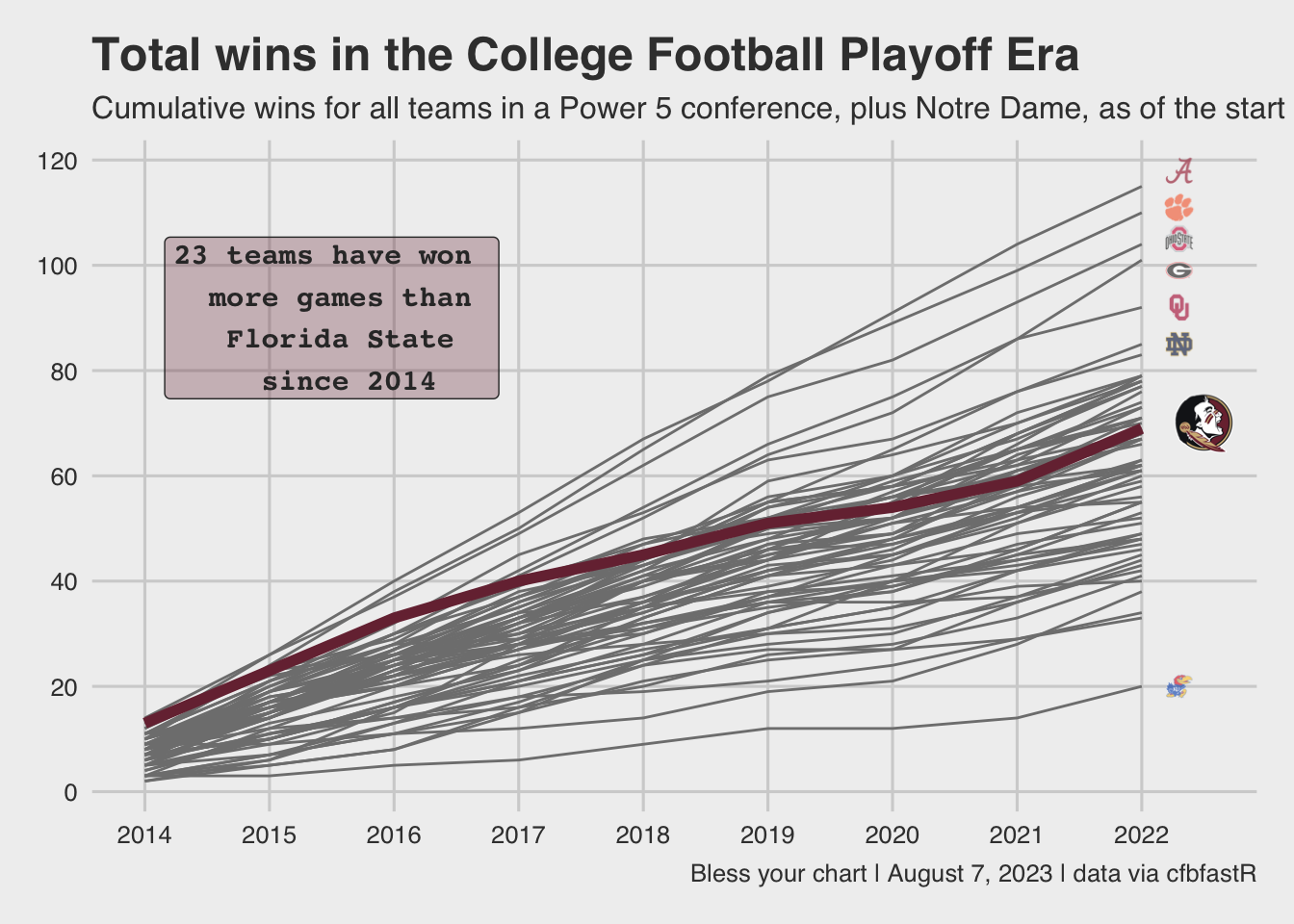
  ggplot2::labs(
    title = "Total wins in the College Football Playoff Era",
    subtitle = "Cumulative wins for all teams in a Power 5 conference, plus Notre Dame, as of the start of the 2023 season.",
    caption = "Bless your chart | August 7, 2023 | data via cfbfastR",
    x = "Year",
    y = "Wins"
  ) +
  ggthemes::theme_fivethirtyeight() +
  ggplot2::theme(legend.position = "none")


# save it
ggplot2::ggsave(
  "fsu.png",
  fsu_plot,
  w = 10,
  h = 10,
  dpi = 600,
  type = 'cairo'
)

fsu_plot