033: NCAA Baseball Tournament Geography

Load data

bracket <- read_csv("bracket2023.csv")

calculate_distance <- function(lat1, lon1, lat2, lon2) {
  if (is.na(lat1) || is.na(lon1) || is.na(lat2) || is.na(lon2)) {
    return(NA)
  }
  if (lat1 == lat2 & lon1 == lon2) {
    return(0)
  } else {
    dist <- distHaversine(c(lon1, lat1), c(lon2, lat2))
    dist_miles <- dist * 0.000621371
    return(dist_miles)
  }
}


# Apply the calculate_distance function to each row of the data frame
bracket <- bracket %>%
  mutate(distance = pmap_dbl(list(latitude, longitude, dest_lat, dest_long), calculate_distance))

# load the bracket data with distances 
blocs <- read_csv("bracket_locations.csv")

Build the maps

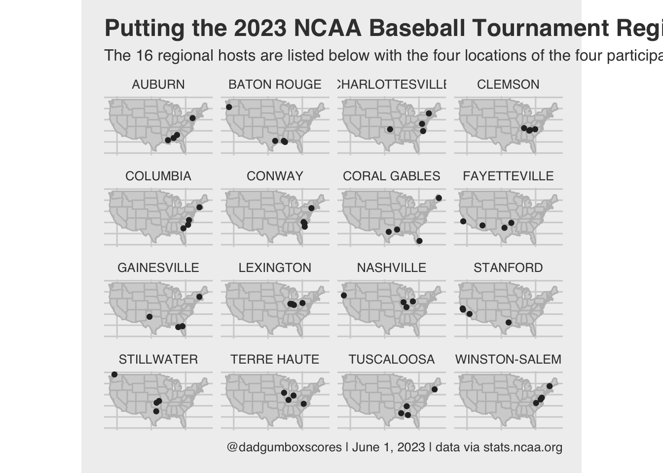
# make plot 
us_map <- map_data("state")

plot <- ggplot() +
  geom_polygon(data = us_map, aes(x = long, y = lat, group = group), fill = "lightgray", color = "gray") +
  coord_fixed(1.3)


reg_plot <- plot +
  geom_jitter(data = bracket, width = 1, height = 2, 
              aes(x = longitude, y = latitude), color = "#2C2C2C", size = 1.5) + 
  facet_wrap(~regional) + 
  theme_fivethirtyeight() +
  labs(
    title = "Putting the 2023 NCAA Baseball Tournament Regionals on a Map",
    subtitle = "The 16 regional hosts are listed below with the four locations of the four participating teams.",
    caption = "@dadgumboxscores | June 1, 2023 | data via stats.ncaa.org"
  )  +
  theme(legend.position = "none", panel.grid = element_blank(),
        axis.title.x=element_blank(), axis.text.x=element_blank(),
        axis.ticks.x=element_blank(), axis.title.y=element_blank(), axis.text.y=element_blank(),
        axis.ticks.y=element_blank())



ggsave(
  "reg_plot.png",
  reg_plot,
  w = 8.5,
  h = 6.5,
  dpi = 600,
  type = 'cairo'
)

reg_plot

Make GT Tables Two Column

tab1 <- blocs %>%
  select(regional, seed, team, conf, distance) %>% 
  arrange(regional, seed) %>% 
  slice(1:32) %>%
  gt::gt(groupname_col = "regional") %>%
  gt::cols_label(
    # rename columns
    seed = "",
    team = "Team",
    conf = "Conference",
    distance = "Distance (miles)",
  ) %>%
  gt::fmt_number(columns = distance,
                 decimals = 0,
                 use_seps = FALSE) %>%
  gtExtras::gt_theme_dot_matrix() %>%
  tab_options (
    source_notes.font.size = px(10),
    row.striping.background_color = '#ffffed',
    table.font.size = px(10),
    column_labels.text_transform = 'capitalize'
  )

tab2 <- blocs %>%
  select(regional, seed, team, conf, distance) %>% 
  arrange(regional, seed) %>% 
  slice(33:64) %>%
  gt::gt(groupname_col = "regional") %>%
  gt::cols_label(
    # rename columns
    seed = "",
    team = "Team",
    conf = "Conference",
    distance = "Distance (miles)",
  ) %>%
  gt::fmt_number(columns = distance,
                 decimals = 0,
                 use_seps = FALSE) %>%
  gtExtras::gt_theme_dot_matrix() %>%
  tab_options (
    source_notes.font.size = px(10),
    row.striping.background_color = '#ffffed',
    table.font.size = px(10),
    column_labels.text_transform = 'capitalize'
  )


listed_tables <- list(tab1, tab2)

obj <- htmltools::div(html("<span style='font-size:15pt; font-weight:bold; font-family:Courier;'><center>2023 NCAA Baseball Tournament Regionals<center></span>"),
                      html("<span style='font-size:9.5pt; font-weight:normal'; font-family:'Courier'><center>@dadgumboxscores | June 1, 2023 | data via stats.ncaa.org<center></span>"),
                      gt_two_column_layout(listed_tables))


gtsave_extra(obj, filename = "table.png", vheight = 875, vwidth = 675)