031: RPI Area charts

Load data + modify tier function

rpi_ranks <- function(url) {
  
  rpi_page <- read_html(url)
  
  rpi_rk <- rpi_page %>%
    html_nodes("table") %>%
    .[1] %>%
    html_table(fill = TRUE)
  
  rpi_table <- as.data.frame(rpi_rk) 
  
  rpi_table <- rpi_table %>% 
    mutate(record = str_split(WL, "-", simplify = T),
           wins = record[,1],
           losses = record[,2]
    ) %>%
    filter(Conference == "ACC") %>%
    select(Team, Conference, RPI)
}

# april 16
rpi_one <- rpi_ranks(url = "https://stats.ncaa.org/selection_rankings/nitty_gritties/31809") %>% mutate(date = 1)

# april 23
rpi_two <- rpi_ranks(url = "https://stats.ncaa.org/selection_rankings/nitty_gritties/31949") %>% mutate(date = 2)

# april 30
rpi_three <- rpi_ranks(url = "https://stats.ncaa.org/selection_rankings/nitty_gritties/32129") %>% mutate(date = 3)

# may 7 
rpi_four <- rpi_ranks(url = "https://stats.ncaa.org/selection_rankings/nitty_gritties/32142") %>% mutate(date = 4)

# may 15
rpi_five <- rpi_ranks(url = "https://stats.ncaa.org/selection_rankings/nitty_gritties/32428") %>% mutate(date = 5)

all_rpi <- bind_rows(rpi_one, rpi_two, rpi_three, rpi_four, rpi_five) %>% 
           mutate(Team = if_else(Team == "Miami (FL)", "Miami", Team))

Build the area chart

# make plot 
all_rpi %>% ggplot(aes(x = date, y = RPI)) + 
  geom_area(aes(fill = Team), linewidth = 2) +
  scale_fill_cfb(alpha = .8) +
    scale_x_continuous(breaks = c(1, 5), labels = c("April 16", "May 14")) + 
    scale_y_reverse(breaks = seq(0, 100, 15)) + 
  facet_wrap( ~Team, nrow = 2) +
  theme_fivethirtyeight() +
  theme(
    strip.text = element_cfb_logo(size = 1),
    plot.title = element_markdown(),
    plot.subtitle = element_markdown(),
    text = element_text(family = "Arial"),
    panel.grid = element_blank(),
    axis.text.x = element_blank()
  ) +
  labs(
    x = "",
    y = "",
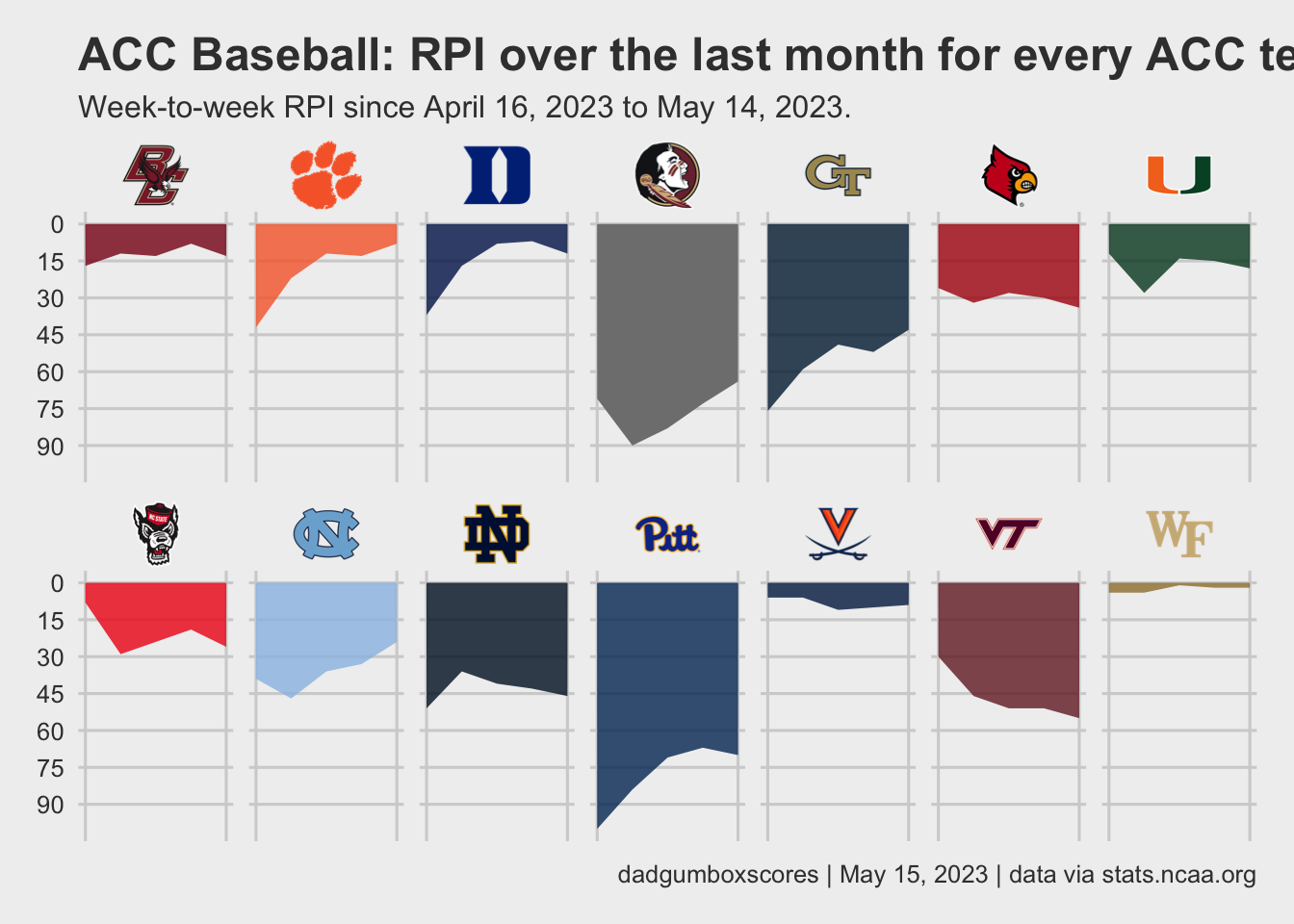
    title = "ACC Baseball: RPI over the last month for every ACC team",
    subtitle = "Week-to-week RPI since April 16, 2023 to May 14, 2023.",
    caption = "dadgumboxscores | May 15, 2023 | data via stats.ncaa.org"
  ) -> rpi_plot

# save it
ggplot2::ggsave(
  "rpi_plot.png",
  rpi_plot,
  w = 10.5,
  h = 6.5,
  dpi = 600,
  type = 'cairo'
)

rpi_plot