030: State/UNC Baseball

geom_col
geom_step
ggthemes
Published

May 10, 2023

Load data + modify tier function

Code
# load csv
stater <- readr::read_csv("state-unc.csv")

# load csv
st_tb <- readr::read_csv("table-st.csv")

# manipulate data 
unc_ncsu <-
  stater %>% 
  dplyr::group_by(location, result) %>% 
  dplyr::count() %>% 
  dplyr::mutate(
    logo = if_else(result == "L", "NC State", "North Carolina"),
    loc_label = case_match(
      location,
      "Away" ~ "West Raleigh",
      "Home" ~ "Chapel Hill",
      location ~ location
    )
  )

Build the area chart

Code
# make plot 
unc_ncsu %>%
  ggplot2::ggplot(aes(x = result, y = n)) +
  ggplot2::geom_col(aes(fill = logo, color = logo), linewidth = 0.005) +
  cfbplotR::geom_cfb_logos(aes(team = logo), width = 0.35, vjust = 0.55) +
  ggplot2::facet_grid( ~ factor(loc_label)) +
  ggplot2::scale_y_continuous(breaks = seq(0, 7, 1)) +
  cfbplotR::scale_fill_cfb(alpha = .8) +
  cfbplotR::scale_color_cfb(alt_colors = unc_ncsu$logo) +
  labs(
    x = "Wins",
    y = "",
    title = "<span style='color:#56a0d3;'>North Carolina</span> is 18-13 against <span style='color:#CC0000;'>NC State</span> since 2013",
    subtitle = "<span style='color:#CC0000;'>5-7</span> in Chapel Hill  \n<span style='color:#56a0d3;'>6-2</span> neutral sites (Omaha, Durham, Greensboro, Charlotte, Louisville)  \n<span style='color:#56a0d3;'>7-4</span> in West Raleigh",
    caption = "dadgumboxscores | May 10, 2023 | data via goheels.com"
  ) +
  ggthemes::theme_solarized() +
  ggplot2::theme(
    plot.title = ggtext::element_markdown(),
    plot.subtitle = ggtext::element_markdown(),
    text = element_text(family = "Arial"),
    panel.grid = element_blank(),
    axis.text.y = element_blank(),
    axis.text.x = element_blank()
  ) -> car_st_plot

# save it
ggplot2::ggsave(
  "car_st_plot.png",
  car_st_plot,
  w = 6.5,
  h = 6.5,
  dpi = 600,
  type = 'cairo'
)

car_st_plot

Build the step chart

Code
stater_long <- stater %>%
  tidyr::pivot_longer(cols = c(unc, state),
                      names_to = "team",
                      values_to = "score")

stater_long %>%
  ggplot2::ggplot(aes(x = season)) +
  ggplot2::geom_step(
    data = stater_long %>% filter(team == "unc"),
    mapping = aes(y = cumsum(score)),
    linewidth = 1,
    color = "#56a0d3"
  ) +
  ggplot2::geom_step(
    data = stater_long %>% filter(team == "state"),
    mapping = aes(y = cumsum(score)),
    linewidth = 1,
    color = "#CC0000"
  ) +
  ggplot2::annotate(
    cfbplotR::GeomCFBlogo,
    x = 2017 ,
    y = 105,
    team = "North Carolina",
    height = .095
  ) +
  ggplot2::annotate(
    cfbplotR::GeomCFBlogo,
    x = 2021 ,
    y = 150,
    team = "NC State",
    height = .095
  ) +
  ggplot2::scale_y_continuous(breaks = seq(0, 165, 15), limits = c(0, 165)) +
  ggplot2::scale_x_continuous(breaks = seq(2013, 2022, 1)) +
  ggthemes::theme_fivethirtyeight() +
  ggplot2::theme(
    text = element_text(family = "Arial", size = 14),
    plot.title = ggtext::element_markdown(),
    plot.subtitle = ggtext::element_markdown()
  ) +
  labs(
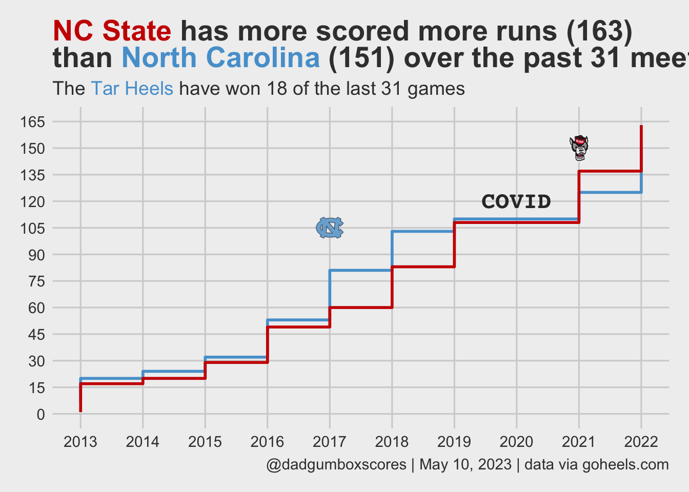
    title = "<span style='color:#CC0000'>NC State</span> has more scored more runs (163)  \nthan <span style='color:#56a0d3'>North Carolina</span> (151) over the past  31 meetings", 
    subtitle = "The <span style='color:#56a0d3'>Tar Heels</span> have won 18 of the last 31 games",
    caption = "@dadgumboxscores | May 10, 2023 | data via goheels.com",
    x = "",
    y = "Runs"
  ) + 
  annotate(
    geom = "text",
    x = 2020,
    y = 120,
    color = "#333333",
    label = "COVID",
    size = 6,
    fontface = 'bold',
    family = 'mono'
  ) -> st_run_plot

# save it
ggplot2::ggsave(
  "st_run_plot.png",
  st_run_plot,
  w = 8.5,
  h = 8.5,
  dpi = 600,
  type = 'cairo'
)

st_run_plot

Make the GT table

Code
st_tb %>%
  dplyr::mutate(Diff = UNC - State) %>%
  dplyr::select(Season, Result, UNC, State, Diff, Location, Type) %>%
  janitor::adorn_totals() %>%
  dplyr::mutate(across(everything(), ~ replace(.x, is.na(.x), ""))) %>%
  gt::gt() %>%
  gt::cols_label(# rename columns
    Type = "",
    Diff = "+/-",) %>%
  gt::fmt(
    columns = c(Diff),
    fns = function(x) {
      ifelse(x > 0, paste0("+", x), x)
    }
  ) %>%
  gt::tab_header(title = "Carolina is 18-13 against State since 2013") %>%
  gt::tab_source_note(source_note = "@dadgumboxscores | May 10, 2023 | data via goheels.com")  %>%
  gtExtras::gt_theme_dot_matrix() %>%
  gt::tab_options (
    source_notes.font.size = px(10),
    row.striping.background_color = '#d0e4f3',
    table.font.size = px(10),
    column_labels.text_transform = 'capitalize'
  ) -> st_table


st_table
Carolina is 18-13 against State since 2013
Season Result UNC State +/- Location
2013 W 7 1 +6 Raleigh Regular
2013 L 3 7 -4 Raleigh Regular
2013 W 2 1 +1 Durham ACC Tournament (18 innings)
2013 L 1 8 -7 Omaha College World Series
2013 W 7 0 +7 Omaha College World Series
2014 W 4 3 +1 Durham ACC Tournament
2015 W 2 1 +1 Chapel Hill Regular
2015 W 3 2 +1 Chapel Hill Regular (10 innings)
2015 L 3 6 -3 Chapel Hill Regular
2016 L 4 6 -2 Raleigh Regular
2016 W 16 4 +12 Raleigh Regular
2016 L 1 10 -9 Raleigh Regular
2017 W 7 2 +5 Chapel Hill Regular
2017 W 7 1 +6 Chapel Hill Regular
2017 L 2 4 -2 Chapel Hill Regular
2017 W 12 4 +8 Louisville ACC Tournament
2018 L 3 8 -5 Durham Non-conference
2018 W 6 5 +1 Raleigh Regular
2018 W 8 6 +2 Raleigh Regular
2018 W 5 4 +1 Raleigh Regular
2019 W 5 3 +2 Chapel Hill Regular
2019 L 2 11 -9 Chapel Hill Regular
2019 L 0 11 -11 Chapel Hill Regular
2021 L 2 9 -7 Chapel Hill Regular
2021 L 1 6 -5 Chapel Hill Regular
2021 L 3 8 -5 Chapel Hill Regular
2021 W 9 6 +3 Charlotte ACC Tournament
2022 W 8 7 +1 Raleigh Regular
2022 L 2 9 -7 Raleigh Regular
2022 W 7 5 +2 Raleigh Regular
2022 W 9 5 +4 Charlotte ACC Tournament
Total - 151 163 -12 - -
@dadgumboxscores | May 10, 2023 | data via goheels.com