027: Women’s Tennis

Load data

# load csv 
ita <- read_csv("ita_april_18_w.csv")

# isolate only the UNC players for the inset table 
unc_tenn <-
  ita %>% filter(Team == "UNC Chapel Hill") %>% 
  select(Rank, Players, `W - L`, Points)

# make cleaner table 
edit_table <- unc_tenn %>% 
    mutate(Players = gsub("([a-z])([A-Z])", "\\1 \\2", Players),
           record = str_split(`W - L`, "-", simplify = T),
           W = record[, 1],
           L = record[, 2]) %>% 
    select(Rank, Players, W, L, Points) %>% 
    mutate_at(vars(-Players), as.numeric) %>% 
    rename(Player = Players)

Set the theme for the plot

# theme
theme_me <- function () {
  theme_minimal(base_size = 10, base_family = "RobotoCondensed-Regular") %+replace%
    theme (
      plot.title = element_text(
        hjust = 0.5,
        size = 18,
        face = "bold",
        lineheight = 0.75,
      ),
      plot.subtitle = element_text(
        hjust = 0.5,
        size = 10,
        lineheight = 0.25,
        vjust = -3,
      ),
      plot.caption = element_text(
        hjust = 1,
        size = 8,
        lineheight = 0.35,
        margin = margin(t = 20)
      ),
      panel.grid.minor = element_blank(),
      plot.background = element_rect(fill = "floral white", color = "floral white")
    )
}

Create scatterplot with inset table

w_ten <- ita %>% mutate(color = if_else(Team == "UNC Chapel Hill", "unc", "not-unc")) %>% 
  ggplot(aes(x = Points, y = Rank, color = color)) + 
  geom_point(aes(size = factor(color))) + 
  scale_color_manual(values = c("#d5d5d5", "#56a0d3")) + 
  scale_x_continuous(breaks=seq(0, 75,25), limits = c(0,75)) +
  scale_y_continuous(breaks=seq(0, 125,25), limits = c(0,125)) +
  annotate(
    geom = "table",
    x = 65,
    y = 45,
    label = list(edit_table),
    table.theme = ttheme_gtbw(colhead = list(bg_params = list(fill = "floralwhite")),
                              core = list(bg_params = list(fill = "floralwhite")),
    size = 1)
  ) + theme_me() + 
  theme(legend.position = "none", plot.title = element_markdown()) + 
  labs(
    x = "Points",
    y = "Rank",
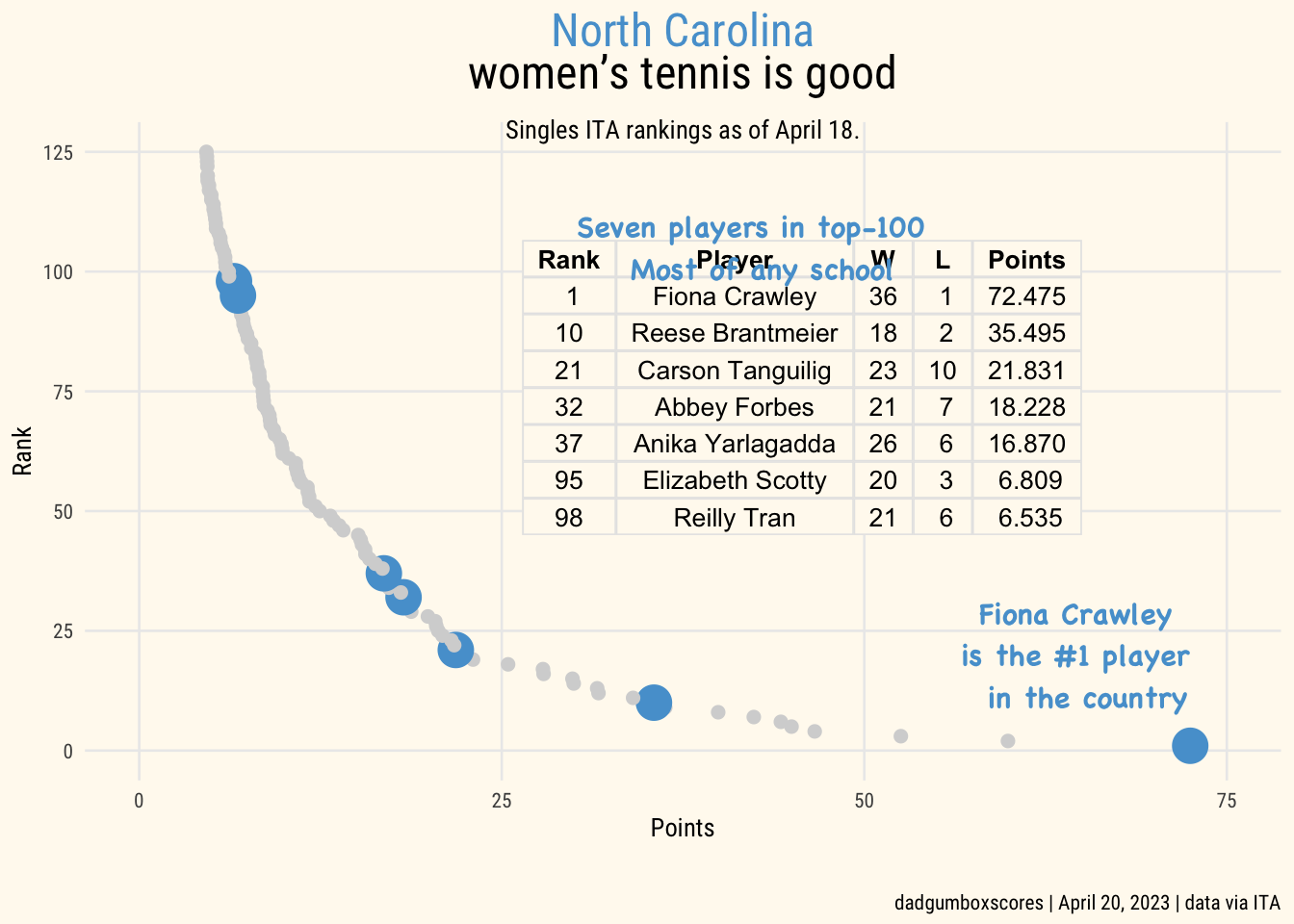
    title = "<span style='color:#56a0d3;'>North Carolina</span>  \nwomen's tennis is good", 
    subtitle ="Singles ITA rankings as of April 18.",
    caption = "dadgumboxscores | April 20, 2023 | data via ITA"
  ) +
  annotate(
    "text",
    x = 65,
    y = 20,
    label = "Fiona Crawley \n is the #1 player  \n in the country",
    family = "Chalkboard Bold",
    size = 4,
    color = "#56a0d3"
  ) +
  annotate(
    "text",
    x = 43,
    y = 105,
    label = "Seven players in top-100  \nMost of any school",
    family = "Chalkboard Bold",
    size = 4,
    color = "#56a0d3"
  )

# save it
ggsave(
    "w_plot.png",
    w_ten,
    w = 6,
    h = 6,
    dpi = 600,
    type = 'cairo'
)

w_ten