020: Pace

Load data

# load december
gp <- read_csv("03_to_23.csv")

# find mean pace 
gp %>% 
    group_by(coach) %>% 
    summarise(mean = mean(pace))

# A tibble: 2 × 2
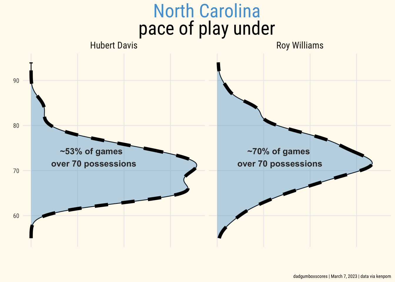
  coach         mean
  <chr>        <dbl>
1 Hubert Davis  70.1
2 Roy Williams  72.7

# 70.1 davis
# 72.7 williams

# find record over last 70
gp %>% 
   slice(579:648) %>% 
   group_by(wl) %>% 
   count()

# A tibble: 2 × 2
# Groups:   wl [2]
  wl        n
  <chr> <int>
1 L        32
2 W        38

# 1 L        32
# 2 W        38

# find same time frame
gp %>% 
    filter(pace < 70 & season > 2017) %>% 
    group_by(coach) %>% 
    count()

# A tibble: 2 × 2
# Groups:   coach [2]
  coach            n
  <chr>        <int>
1 Hubert Davis    33
2 Roy Williams    33

# 1 Hubert Davis    33
# 2 Roy Williams    33

  ann_dat_text<-data.frame(
    coach=c("Hubert Davis","Roy Williams"),
    pace=c(0.040,70),
    label=c("~53% of games  \nover 70 possessions","~70% of games \nover 70 possessions")
)

Set the theme for the plot

# theme
  theme_me <- function () {
    theme_minimal(base_size = 10, base_family = "RobotoCondensed-Regular") %+replace%
      theme (
        plot.title = element_text(
          hjust = 0.5,
          size = 24,
          face = "bold"
        ),
        plot.subtitle = element_text(
          hjust = 0.5,
          size = 10,
          lineheight = 0.25,
          vjust = -0.5
        ),
        plot.caption = element_text(
          hjust = 1,
          size = 6,
          lineheight = 0.35,
          margin = margin(t = 20)
        ),
        panel.grid.minor = element_blank(),
        plot.background = element_rect(fill = "floral white", color = "floral white")
      )
  }

Create density plot

dense <- gp %>% 
    ggplot() + 
    aes(x = pace) +
    geom_density() +
    geom_density(fill="#56a0d3", 
                 size = 2,
                 position="identity",
                 alpha = 0.4,
                 linetype = "dashed")+
    coord_flip() +
   facet_grid(. ~ coach) +
    theme_me() +
theme(legend.position = "none", plot.title = element_markdown(),
    axis.ticks.y = element_blank(),
    axis.ticks.x = element_blank(),
    axis.text.x = element_blank(),
    strip.text.x = element_markdown(size = 12, face = "bold")
  ) + 
labs(
    x = "",
    y = "",
    title = "<span style='color:#56a0d3;'>North Carolina</span>  \npace of play \nunder",
    caption = "dadgumboxscores | March 7, 2023 | data via kenpom"
  ) + geom_text(
    data = ann_dat_text,
    y = 0.027,
    x = 73,
    label=ann_dat_text$label,
    color = "#333333",
    fontface = "bold"
)

# save it
ggsave(
  "dense.png",
  dense,
  w = 6,
  h = 8,
  dpi = 600,
  type = 'cairo'
)

dense