close_table <- close %>%arrange(-Season) %>%gt() %>%cols_label(# rename columnsPct ="Win %",) %>%fmt_number(columns = Pct,decimals =1,use_seps =FALSE) %>%gt_theme_dot_matrix() %>%tab_header(title =md("ACC home team record in games decided by 5 or fewer points")) %>%tab_source_note(source_note ="@dadgumboxscores | February 17, 2023 | data via kenpom") %>%tab_options (source_notes.font.size =px(10),row.striping.background_color ='#ffffed',table.font.size =px(10),column_labels.text_transform ='capitalize' )gtsave_extra(close_table,"close_g_table.png",vwidth =275,vheight =275)close_table
ACC home team record in games decided by 5 or fewer points
Season
W
L
Win %
2023
22
15
59.5
2022
25
29
46.3
2021
23
10
69.7
2020
23
28
45.1
2019
19
12
61.3
@dadgumboxscores | February 17, 2023 | data via kenpom
Code
rec_table <- acc_by_team %>%gt() %>%cols_label(# rename columnslogo ="",team ="Team",win_pct ="Win %",) %>%gt_fmt_cfb_logo(columns ="logo") %>%tab_header(title ="ACC Home records by team since 2018-19 season",) %>%tab_source_note(source_note ="@dadgumboxscores | February 17, 2023 | data via kenpom") %>%# adjust font sizestab_options (source_notes.font.size =px(10),table.font.size =px(12), ) %>%# add theme using 538gt_theme_excel()gtsave_extra(rec_table,"rec_table.png",vwidth =650,vheight =650)rec_table
ACC Home records by team since 2018-19 season
Team
W
L
Win %
Virginia
36
8
0.818
Duke
36
9
0.800
Florida State
35
10
0.778
North Carolina
32
12
0.727
Clemson
32
14
0.696
Virginia Tech
27
16
0.628
Syracuse
26
18
0.591
Miami FL
26
20
0.565
Louisville
24
19
0.558
Wake Forest
24
21
0.533
Georgia Tech
24
23
0.511
Notre Dame
23
22
0.511
NC State
22
22
0.500
Pittsburgh
22
24
0.478
Boston College
18
26
0.409
@dadgumboxscores | February 17, 2023 | data via kenpom
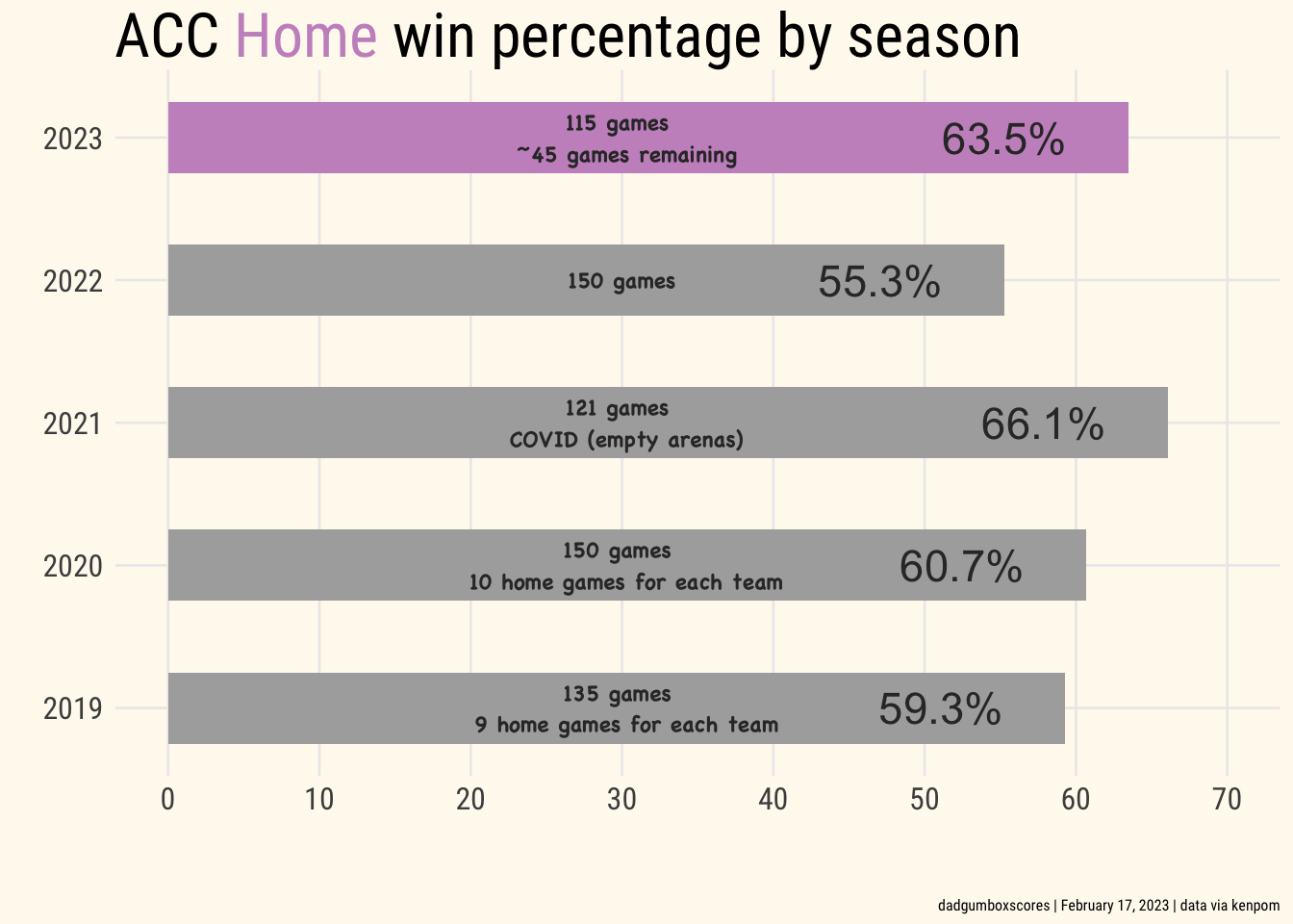
Make the bar plot
Code
wp_plot <- win_pct %>%mutate(color =case_match(Season,2023~"#c994c7",.default ="#acacac")) %>%arrange(-Season) %>%ggplot(aes(Season, WP, fill = color)) +geom_col(width =0.5) +geom_text(aes(label =paste0(WP, "%"), hjust =1.5),color ="#333333",size =6) +coord_flip() +scale_y_continuous(breaks =seq(0, 70, 10), limits =c(0, 70)) +labs(x ="",y ="",title ="ACC <span style='color:#c994c7;'>Home</span> win percentage by season",caption ="dadgumboxscores | February 17, 2023 | data via kenpom" ) +theme_me() +scale_fill_identity(guide ="none") +theme(plot.title =element_textbox_simple(), axis.text =element_text(size =12)) +annotate("text",x =2021,y =30,label ="121 games \n COVID (empty arenas)",family ="Chalkboard Bold",size =3,fontface ="bold",color ="#333333", ) +annotate("text",x =2020,y =30,label ="150 games \n 10 home games for each team",family ="Chalkboard Bold",size =3,fontface ="bold",color ="#333333", ) +annotate("text",x =2022,y =30,label ="150 games",family ="Chalkboard Bold",size =3,fontface ="bold",color ="#333333", ) +annotate("text",x =2023,y =30,label ="115 games \n ~45 games remaining",family ="Chalkboard Bold",size =3,fontface ="bold",color ="#333333", ) +annotate("text",x =2019,y =30,label ="135 games \n 9 home games for each team",family ="Chalkboard Bold",size =3,fontface ="bold",color ="#333333", )ggsave("wp.png", wp_plot,w =7.5,h =7.5,dpi =600,type ='cairo')wp_plot