014: Caleb Love true shooting

Load data and manipulate

cl <- kp_player_career(player_id = 50282)

love <- data.frame(cl[[2]]) %>% 
           mutate(tsa = ((fga_2 + fga_3) + (.475 * fta)),
                  ts_pct = pts / (2*tsa),
                  devil = if_else(opponent == "Duke", "Duke", "")
           )

# find true shooting differeces via sports-ref
# https://www.sports-reference.com/cbb/players/caleb-love-1/splits/

Set the themes for the plot

# theme
  theme_me <- function () {
    theme_minimal(base_size = 10, base_family = "RobotoCondensed-Regular") %+replace%
      theme (
        plot.title = element_text(
          hjust = 0.5,
          size = 24,
          face = "bold"
        ),
        plot.subtitle = element_text(
          hjust = 0.5,
          size = 10,
          lineheight = 0.25,
          vjust = -0.5
        ),
        plot.caption = element_text(
          hjust = 1,
          size = 6,
          lineheight = 0.35,
          margin = margin(t = 20)
        ),
        panel.grid.minor = element_blank(),
        plot.background = element_rect(fill = "floral white", color = "floral white")
      )
  }

Make the bar plot

love_plot <- love %>% 
ggplot(aes(x = year, y = ts_pct, color = devil)) +
geom_beeswarm(dodge.width=0.5, size = 4) +
scale_x_continuous(breaks = seq(2021, 2023, 1)) + 
scale_y_continuous(breaks = seq(0, 0.90, 0.10), labels = c(0, 10, 20, 30, 40, 50, 60, 70, 80, 90), limits = c(0, .90)) +
scale_color_manual(values = c("lightpink", "#00539B")) + 
theme_me() +
theme(legend.position = "none", plot.title = element_markdown()) + 
labs(
    x = "",
    y = "",
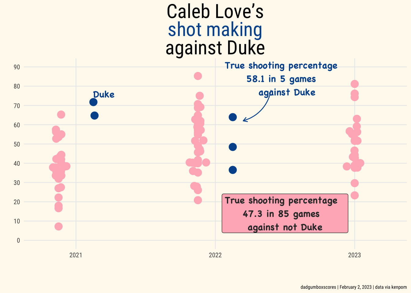
    title = "Caleb Love's  \n<span style='color:#00539B;'>shot making</span>  \nagainst Duke",
    caption = "dadgumboxscores | February 2, 2023 | data via kenpom"
  ) +
  annotate(
    "text",
    x = 2021.2,
    y = 0.76,
    label = "Duke",
    family = "Chalkboard Bold",
    size = 4,
    fontface = "bold",
    color = "#00539B",
  ) +
    annotate(
    "text",
    x = 2022.5,
    y = 0.84,
    label = "True shooting percentage  \n58.1 in 5 games  \n against Duke",
    family = "Chalkboard Bold",
    size = 4,
    fontface = "bold",
    color = "#00539B"
  ) +
  annotate(
    geom = "curve",
    color = "#00539B",
    x = 2022.4,
    y = 0.78,
    xend = 2022.2,
    yend = 0.62,
    curvature = -.3,
    arrow = arrow(length = unit(2, "mm"))
  ) +
annotate(
    "label",
    x = 2022.5,
    y = 0.14,
    label = "True shooting percentage  \n47.3 in 85 games  \nagainst not Duke",
    family = "Chalkboard Bold",
    size = 4,
    color = "#333333",
    fontface = "bold",
    fill = "lightpink"
  )

# save it
ggsave(
  "love_plot.png",
  love_plot,
  w = 6,
  h = 8,
  dpi = 300,
  type = 'cairo'
)

love_plot