011: Directors’ Cup

Load data and manipulate

dc_rank <- read_csv("dc_ranks.csv")

fbs <- dc_rank %>%
  filter(Division == "FBS" & fall_final > 99) %>%
  select(-c(Division, fall_final)) %>%
  select(-contains(c("rank"))) %>%
  rename("Team" = Institution) %>%
  mutate(non_fb_pts = rowSums(select(., ends_with("pts")))) %>%
  mutate(
    non_fb_pts = (non_fb_pts - fb_pts),
    Team = case_when(
      Team == "Miami (FL)" ~ "Miami",
      Team == "North Carolina State" ~ "NC State",
      TRUE ~ Team
    )
  ) %>%
  select(Team, Conference, non_fb_pts, fb_pts)

Set the themes for the plot

# theme
  theme_me <- function () {
    theme_minimal(base_size = 10, base_family = "RobotoCondensed-Regular") %+replace%
      theme (
        plot.title = element_text(
          hjust = 0.5,
          size = 24,
          face = "bold"
        ),
        plot.subtitle = element_text(
          hjust = 0.5,
          size = 10,
          lineheight = 0.25,
          vjust = -0.5
        ),
        plot.caption = element_text(
          hjust = 1,
          size = 6,
          lineheight = 0.35,
          margin = margin(t = 20)
        ),
        panel.grid.minor = element_blank(),
        plot.background = element_rect(fill = "floral white", color = "floral white")
      )
  }

Make the scatterplot with the logos

dc_plot <- fbs %>%
  ggplot(aes(x = fb_pts, y = non_fb_pts)) +
  geom_cfb_logos(aes(team = Team), width = 0.038, postion = "jitter") +
  scale_x_continuous(breaks = seq(0, 100, 25), limits = c(0, 100)) +
  scale_y_continuous(breaks = seq(0, 375, 25), limits = c(0, 375)) +
  geom_vline(xintercept = 15,
             linetype = 'dashed',
             color = "#333333") +
  theme_me() +
  labs(
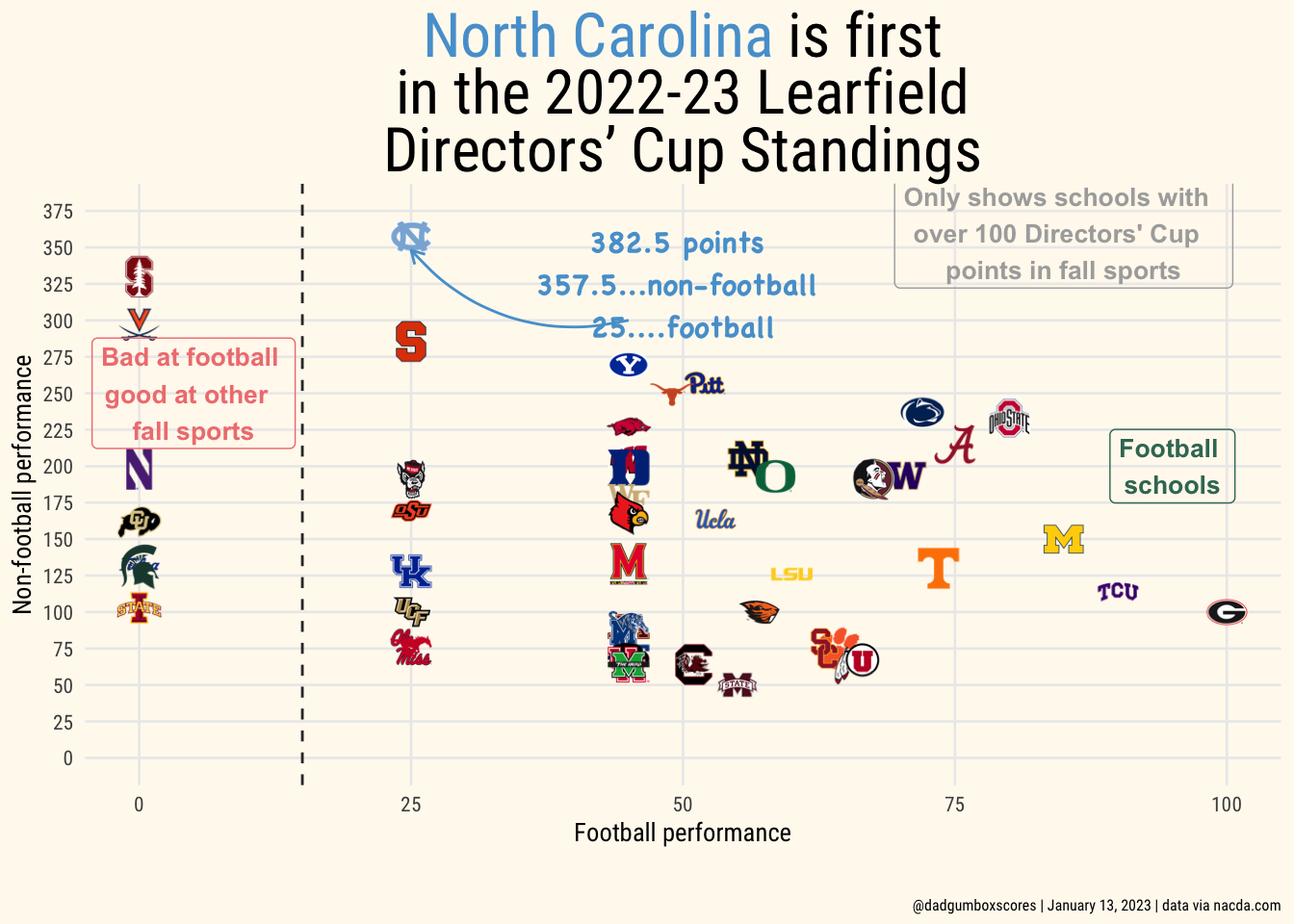
    title = "<span style='color:#56a0d3'>North Carolina</span> is first  \nin the 2022-23 Learfield  \nDirectors' Cup Standings",
    caption = "@dadgumboxscores | January 13, 2023 | data via nacda.com",
    x = "Football performance",
    y = "Non-football performance"
  ) +
  theme(legend.position = "none", plot.title = element_markdown()) +
  annotate(
    geom = 'label',
    y = 250,
    x = 5,
    label = "Bad at football \ngood at other  \nfall sports",
    fontface = 'bold',
    colour = "#f08080",
    size = 3.5,
    fill = "floral white",
    alpha = 0.1
  ) +
  annotate(
    geom = 'label',
    y = 200,
    x = 95,
    label = "Football \nschools",
    fontface = 'bold',
    colour = "#3b7763",
    size = 3.5,
    fill = "floral white",
    alpha = 0.1
  ) +
  annotate(
    geom = 'label',
    y = 360,
    x = 85,
    label = "Only shows schools with  \nover 100 Directors' Cup  \npoints in fall sports",
    fontface = 'bold',
    colour = "#ababab",
    size = 3.5,
    fill = "floral white",
    alpha = 0.1
  ) +
  annotate(
    "text",
    x = 50,
    y = 325,
    label = "382.5 points \n 357.5...non-football  \n25....football",
    family = "Chalkboard Bold",
    size = 4,
    color = "#56a0d3"
  ) +
  annotate(
    geom = "curve",
    color = "#56a0d3",
    x = 45,
    y = 300,
    xend = 25,
    yend = 348,
    curvature = -.3,
    arrow = arrow(length = unit(2, "mm"))
  )


# save the chart
ggsave(
  "dc_plot.png",
  dc_plot,
  w = 7.5,
  h = 7.5,
  dpi = 600,
  type = 'cairo'
)

dc_plot