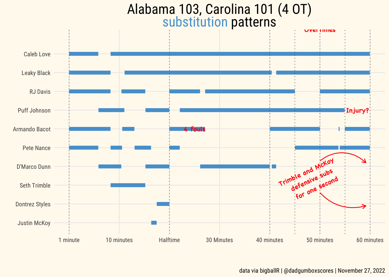
004: Sub Patterns in 60 minutes of basketball

Load data

# data was manually edited due to errors in pbp, but code is still below
bama_data <- read_csv("bama.csv")

# schedule
schedule <- get_team_schedule(season = "2022-23", team.name = "North Carolina")

================================================================================

#' Helper function to get player stints
#' Used in plot_player_stints
#' @import dplyr
get_player_stints <- function(game_data, player_name) {
  home <- player_name %in% unlist(game_data[,4:8])

  cols = if(home) 4:8 else 9:13

  is_on <- apply(game_data[,cols], 1, function(x){player_name %in% x})

  subs <- (is_on) & (lag(is_on) == F) | (is_on == T) & (lead(is_on) == F)
  subs[c(1,length(subs))] <- is_on[c(1,length(subs))]

  stint_data <- game_data %>%
    dplyr::select(Game_Seconds, Home_Score, Away_Score) %>%
    dplyr::mutate(Sub = cumsum(subs)) %>%
    dplyr::group_by(Sub) %>%
    dplyr::summarise(Start = min(Game_Seconds),
              Stop = max(Game_Seconds),
              Score_Dif = max(Home_Score) - min(Home_Score) - max(Away_Score) + min(Away_Score)
    ) %>%
    dplyr::mutate(Score_Dif = if(home) Score_Dif else -Score_Dif,
           Player = player_name,
           Team = home
    ) %>%
    dplyr::filter(Start != Stop, Sub %%2 == 1)

  return(stint_data)
}

# get pbp
bama_pbp <- get_play_by_play(schedule$Game_ID[7])

  game_data <- bama_pbp %>%
    dplyr::filter(Game_Seconds <= 3600) %>%
    dplyr::select(Game_Seconds, Home_Score, Away_Score, Home.1:Away.5) %>%
    tidyr::complete(Game_Seconds = 0:3600) %>%
    dplyr::mutate(First = Game_Seconds <= 1200) %>%
    dplyr::group_by(First) %>%
    tidyr::fill(-First, .direction = "up") %>%
    dplyr::ungroup() %>%
    dplyr::select(-First) %>%
    dplyr::distinct() %>%
    dplyr::select(Game_Seconds, Home_Score, Away_Score, dplyr::everything())

players <- unique(unlist(game_data[,4:13]))
players <- players[!is.na(players)]

  all_stints <- lapply(players, get_player_stints, game_data = game_data) %>%
    dplyr::bind_rows() %>%
    dplyr::mutate(
      Player = reorder(Player, -Start, FUN = max)
    )

bama_data <- all_stints %>% 
        filter(Team == FALSE) %>%
        mutate(Player = str_replace(Player, "^\\S* ", "")) %>%
        mutate(Stint = (Stop - Start)) %>%
        group_by(Player) %>%
        mutate(Time = sum(Stint)) %>%
        ungroup() %>% 
        arrange(-Time) %>% 
        mutate(Opponent = 'Alabama') %>%
        mutate(Player = case_when(
          Player == "PETE.NANCE" ~ "Pete Nance",
          Player == "RJ.DAVIS" ~ "RJ Davis",
          Player == "CALEB.LOVE" ~ "Caleb Love",
          Player == "LEAKY.BLACK" ~ "Leaky Black",
          Player == "ARMANDO.BACOT" ~ "Armando Bacot",
          Player == "SETH.TRIMBLE" ~ "Seth Trimble", 
          Player == "DMARCO.DUNN" ~ "D'Marco Dunn",
          Player == "TYLER.NICKEL" ~ "Tyler Nickel", 
          Player == "DONTREZ.STYLES" ~ "Dontrez Styles",
          Player == "PUFF.JOHNSON" ~ "Puff Johnson",
          Player == "WILLIAM.SHAVER" ~ "Will Shaver",
          Player == "JUSTIN.MCKOY" ~ "Justin McKoy",))

Set the theme for the plot

# theme
theme_me <- function () {
  theme_minimal(base_size = 10, base_family = "RobotoCondensed-Regular") %+replace%
    theme (
      plot.title = element_text(
        hjust = 0.5,
        size = 18,
        face = "bold",
        lineheight = 0.75,
      ),
      plot.subtitle = element_text(
        hjust = 0.5,
        size = 10,
        lineheight = 0.25,
        vjust = -3,
      ),
      plot.caption = element_text(
        hjust = 1,
        size = 8,
        lineheight = 0.35,
        margin = margin(t = 20)
      ),
      panel.grid.minor = element_blank(),
      plot.background = element_rect(fill = "floral white", color = "floral white")
    )
}

Create the plot

# make the plot
bama <- ggplot2::ggplot(bama_data) +
    ggplot2::geom_linerange(ggplot2::aes(x= fct_reorder(Player, Time), ymin = Start, ymax = Stop), size = 2.4, color = "#56a0d3") +
    coord_flip() + 
    ggplot2::scale_y_continuous(breaks = c(0,600, 1200, 1800, 2400, 3000, 3600), 
    labels = c("1 minute", "10 minutes", "Halftime", "30 Minutes", "40 minutes", "50 minutes", "60 minutes")) +
    ggplot2::geom_hline(yintercept = c(0,1200,2400,2700,3000,3300,3600), color = "gray30", linetype ="dotted", size = 0.3) +
    theme_me() + 
  theme(plot.title = element_markdown()) +
  labs(
    x = "",
    y = "",
    title = "Alabama 103, Carolina 101 (4 OT)  \n<span style='color:#56a0d3;'>substitution</span> patterns",
    caption = "data via bigballR | @dadgumboxscores | November 27, 2022"
  ) +
  annotate(
    "text",
    x = 6,
    y = 1500,
    label = "4 fouls",
    family = "Chalkboard Bold",
    size = 3,
    color = "red"
  ) +
annotate(
    "text",
    x = 3.3,
    y = 2900,
    label = "Trimble and McKoy \n defensive subs \n for one second",
    family = "Chalkboard Bold",
    size = 3,
    color = "red",
    angle = 25
  ) +
annotate(
    "text",
    x = 11.3,
    y = 3000,
    label = "Overtimes",
    family = "Chalkboard Bold",
    size = 3,
    color = "red",
  ) +
annotate(
    geom = "curve",
    color = "red",
    x = 2.6,
    y = 3000,
    xend = 1.9,
    yend = 3550,
    curvature = .3,
    arrow = arrow(length = unit(2, "mm"))
  ) +
annotate(
    geom = "curve",
    color = "red",
    x = 4.3,
    y = 3000,
    xend = 4.2,
    yend = 3550,
    curvature = -.4,
    arrow = arrow(length = unit(2, "mm"))
  ) +
annotate(
    "text",
    x = 7,
    y = 3450,
    label = "Injury?",
    family = "Chalkboard Bold",
    size = 3,
    color = "red",
  )

  # save the plot
  ggsave(
  "alabama.png",
  bama,
  w = 7.5,
  h = 5.5,
  dpi = 300,
  type = 'cairo'
)

  
bama