003: Carolina and State since 1988

Load data

state <- read_csv("state-unc.csv")

Pivot the data and count it

games <- state %>%
pivot_longer(cols = c("Pts", "Opp"), names_to = "team", values_to = "points") %>%
select(Year, team, points) %>%
mutate(team = if_else(team == "Pts", "North Carolina", "NC State")) %>% 
filter(Year > 1987)

Set the theme for the plot

# theme
theme_me <- function () {
  theme_minimal(base_size = 10, base_family = "RobotoCondensed-Regular") %+replace%
    theme (
      plot.title = element_text(
        hjust = 0.5,
        size = 18,
        face = "bold",
        lineheight = 0.75,
      ),
      plot.subtitle = element_text(
        hjust = 0.5,
        size = 10,
        lineheight = 0.25,
        vjust = -3,
      ),
      plot.caption = element_text(
        hjust = 1,
        size = 8,
        lineheight = 0.35,
        margin = margin(t = 20)
      ),
      panel.grid.minor = element_blank(),
      plot.background = element_rect(fill = "floral white", color = "floral white")
    )
}

Create the plot

# make the plot
state_plot <- games %>%
ggplot(aes(x= team,y= Year, fill = team))+
  geom_point(aes(size=points), shape = 21)+
  scale_fill_manual(values = c("#CC0000", "#56a0d3"), guide = "none") +
  geom_text(color="floral white", size=2.75,
                aes(x=team, y=Year, label=points)) +
 scale_y_continuous(breaks=seq(1988, 2021,1), labels = paste0("`", sprintf('%02d', 1988:2021 %% 100))) +
 theme_me() +
 scale_size(
  limits = c(0,52),
  range = c(4,8.99),
  guide = "none"
) +
geom_hline(yintercept=1997.5, linetype="dashed", 
                color = "#194967", size=1) +
geom_hline(yintercept=2018.5, linetype="dashed", 
                color = "#194967", size=1) +
coord_flip() +
theme(axis.text.y = element_cfb_logo(size = 1.75)) +
labs(
    x = "",
    y = "",
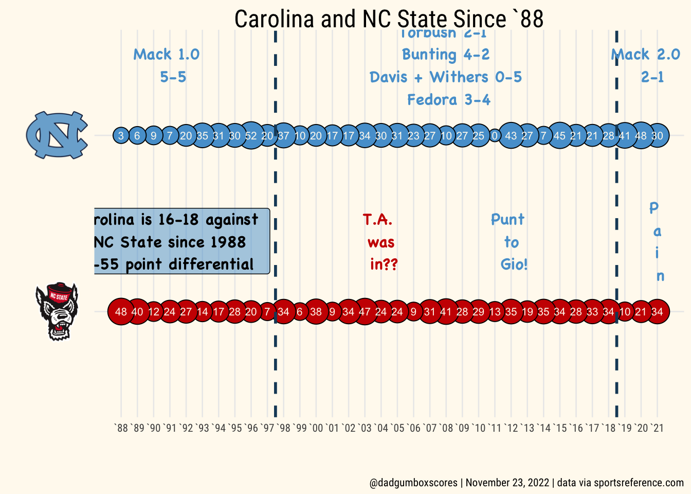
    title = "Carolina and NC State Since `88",
    caption = "@dadgumboxscores | November 23, 2022 | data via sportsreference.com"
  ) 

# add annotations
stater <- state_plot + annotate(
    "text",
    x = 2.4,
    y = 1991,
    label = "Mack 1.0 \n 5-5",
    family = "Chalkboard Bold",
    size = 4,
    color = "#56a0d3"
  ) +
  annotate(
    "text",
    x = 2.4,
    y = 2020.5,
    label = "Mack 2.0 \n 2-1",
    family = "Chalkboard Bold",
    size = 4,
    color = "#56a0d3"
  ) +
  annotate(
    "text",
    x = 2.4,
    y = 2008,
    label = "Torbush 2-1 \n Bunting 4-2 \n Davis + Withers 0-5 \n Fedora 3-4",
    family = "Chalkboard Bold",
    size = 4,
    color = "#56a0d3"
  ) +
  annotate(
    "text",
    x = 1.4,
    y = 2004,
    label = "T.A. \n was \n in??",
    family = "Chalkboard Bold",
    size = 4,
    color = "#CC0000",
  ) +
 annotate(
    "text",
    x = 1.4,
    y = 2012,
    label = "Punt \n to \n Gio!",
    family = "Chalkboard Bold",
    size = 4,
    color = "#56a0d3",
  ) +
   annotate(
    "text",
    x = 1.4,
    y = 2021,
    label = "P \n a \n i \n n",
    family = "Chalkboard Bold",
    size = 4,
    color = "#56a0d3",
  ) +
 annotate(
    geom = 'label',
    x = 1.4,
    y = 1991,
    label = "Carolina is 16-18 against \n NC State since 1988 \n -55 point differential",
    fill = "#56a0d3",
    family = "Chalkboard Bold",
    alpha = .5, 
    size = 4,
  )
  
# save the chart
ggsave(
  "state.png",
  stater,
  w = 10,
  h = 7,
  dpi = 300,
)


  
stater