001: Football drives

Fetch data from cfbfastR

defense <- cfbd_drives(
    2022,
    season_type = "regular",
    defense_team = "North Carolina"
)

# number the games, so we can put them in the right order
defense <- defense %>%
           mutate(game_num = case_when (
            offense == "Florida A&M" ~ 1,
            offense == "Appalachian State" ~ 2,
            offense == "Georgia State" ~ 3,
            offense == "Notre Dame" ~ 4,
            offense == "Virginia Tech" ~ 5,
            offense == "Miami" ~ 6,
            offense == "Duke" ~ 7,
            offense == "Pittsburgh" ~ 8,
            offense == "Virginia" ~ 9,
            offense == "Wake Forest" ~ 10,
           )) %>%
           arrange(game_num) %>%
           mutate(drive_num = 1:n()) %>% 
           select(game_num, offense, drive_num, drive_number, scoring, plays, yards, drive_result)

Factors and theme

def_drive <- defense %>%
       mutate(count = if_else(scoring == "TRUE", 1,1.01)) 
         
def_drive$offense <- factor(def_drive$offense)
def_drive$ymin <- 0 
def_drive$ymax <- 1
def_drive$xmax <- cumsum(def_drive$count)
def_drive$xmin <- c(0, head(def_drive$xmax, n=-1))

Set the theme for the plot

# theme
theme_me <- function () {
  theme_minimal(base_size = 10, base_family = "RobotoCondensed-Regular") %+replace%
    theme (
      plot.title = element_text(
        hjust = 0.5,
        size = 24,
        face = "bold"
      ),
      plot.subtitle = element_text(
        hjust = 0.5,
        size = 10,
        lineheight = 0.25,
        vjust = -0.5
      ),
      plot.caption = element_text(
        hjust = 1,
        size = 6,
        lineheight = 0.35,
        margin = margin(t = 20)
      ),
      panel.grid.minor = element_blank(),
      plot.background = element_rect(fill = "floral white", color = "floral white")
    )
}

Create the plot

defense_plot <- def_drive %>%
  mutate(offense = fct_relevel(offense, c("Florida A&M", "Appalachian State", "Georgia State", "Notre Dame", "Virginia Tech", "Miami", "Duke", "Pittsburgh", "Virginia", "Wake Forest"))) %>% 
  ggplot(aes(x = offense, y = count, fill = count)) +
  geom_bar(stat = "identity", colour = "black") +
  labs(y="Drive number", x = "") +
  scale_y_continuous(breaks = seq(0, 20, 1)) +
  coord_flip() + 
  theme_me() +
  theme(axis.text.y = element_cfb_logo(size = 1), legend.position = "none") +
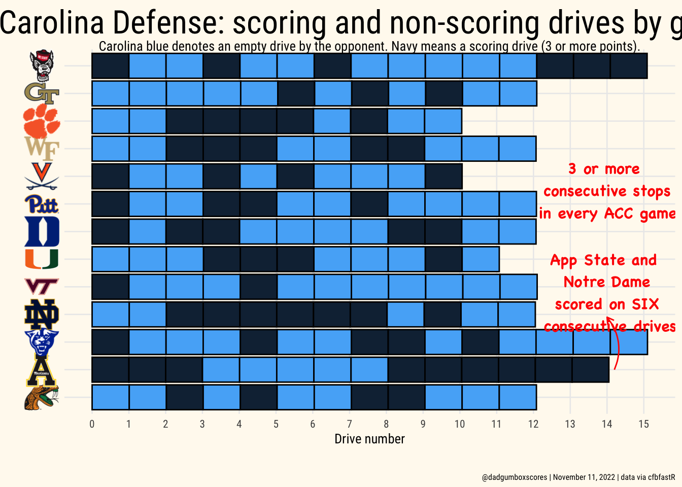
  labs(title = "Carolina Defense: scoring and non-scoring drives by game",
       subtitle = "Carolina blue denotes an empty drive by the opponent. Navy means a scoring drive (3 or more points).",
       caption = "@dadgumboxscores | November 11, 2022 | data via cfbfastR") +
  annotate(
    "text",
    x = 8.5,
    y = 14,
    label = "3 or more \n consecutive stops \n in every ACC game!",
    family = "Chalkboard Bold",
    size = 4,
    color = "red"
  ) + 
  annotate(
    "text",
    x = 4.8,
    y = 14,
    label = "App State and \n Notre Dame \n scored on SIX \n consecutive drives",
    family = "Chalkboard Bold",
    size = 4,
    color = "red"
  ) +
  annotate(
    geom = "curve",
    color = "red",
    x = 2,
    y = 14.2,
    xend = 3.9,
    yend = 14,
    curvature = .3,
    arrow = arrow(length = unit(2, "mm"))
  ) 

# save plot
ggsave(
  "def.png",
  defense_plot,
  w = 10.5,
  h = 7.5,
  dpi = 300,
  type = 'cairo'
)

defense_plot